CIRCUIT SCHEMATIC SYMBOLS

Wires and connections

Older electrical schematics showed connecting wires crossing, while non-connecting wires "jumped" over each other with little half-circle marks. Newer electrical schematics show connecting wires joining with a dot, while non-connecting wires cross with no dot. However, some people still use the older convention of connecting wires crossing with no dot, which may create confusion.

For this reason, I opt to use a hybrid convention, with connecting wires unambiguously connected by a dot, and non-connecting wires unambiguously "jumping" over one another with a half-circle mark. While this may be frowned upon by some, it leaves no room for interpretational error: in each case, the intent is clear and unmistakable:

Power sources

Resistors

Capacitors

Inductors

Mutual inductors

Switches, hand actuated

Switches, process actuated

It is very important to keep in mind that the "normal" contact status of a process-actuated switch refers to its status when the process is absent and/or inactive, not "normal" in the sense of process conditions as expected during routine operation. For instance, a normally-closed low-flow detection switch installed on a coolant pipe will be maintained in the actuated state (open) when there is regular coolant flow through the pipe. If the coolant flow stops, the flow switch will go to its "normal" (unactuated) status of closed.

A limit switch is one actuated by contact with a moving machine part. An electronic limit switch senses mechanical motion, but does so using light, magnetic fields, or other non-contact means.

Switches, electrically actuated (relays)

Connectors

Diodes

Transistors, bipolar

Transistors, junction field-effect (JFET)

Transistors, insulated-gate field-effect (IGFET or MOSFET)

Transistors, hybrid

Thyristors

Integrated circuits

Electron tubes

READ MORE...

PERIODIC TABLE OF THE ELEMENTS

Table (landscape view)

See Figure below.

Periodic table of chemical elements.

Table (portrait view)

Periodic table of chemical elements.

Data

Atomic masses shown in parentheses indicate the most stable isotope (longest half-life) known.

Electron configuration data was taken from Douglas C. Giancoli's Physics, 3rd edition. Average atomic masses were taken from Kenneth W. Whitten's, Kenneth D. Gailey's, and Raymond E. Davis' General Chemistry, 3rd edition. In the latter book, the masses were specified as 1985 IUPAC values.

READ MORE...

TROUBLESHOOTING -- THEORY AND PRACTICE

Perhaps the most valuable but difficult-to-learn skill any technical person could have is the ability to troubleshoot a system. For those unfamiliar with the term, troubleshooting means the act of pinpointing and correcting problems in any kind of system. For an auto mechanic, this means determining and fixing problems in cars based on the car's behavior. For a doctor, this means correctly diagnosing a patient's malady and prescribing a cure. For a business expert, this means identifying the source(s) of inefficiency in a corporation and recommending corrective measures.

Troubleshooters must be able to determine the cause or causes of a problem simply by examining its effects. Rarely does the source of a problem directly present itself for all to see. Cause/effect relationships are often complex, even for seemingly simple systems, and often the proficient troubleshooter is regarded by others as something of a miracle-worker for their ability to quickly discern the root cause of a problem. While some people are gifted with a natural talent for troubleshooting, it is a skill that can be learned like any other.

Sometimes the system to be analyzed is in so bad a state of affairs that there is no hope of ever getting it working again. When investigators sift through the wreckage of a crashed airplane, or when a doctor performs an autopsy, they must do their best to determine the cause of massive failure after the fact. Fortunately, the task of the troubleshooter is usually not this grim. Typically, a misbehaving system is still functioning to some degree and may be stimulated and adjusted by the troubleshooter as part of the diagnostic procedure. In this sense, troubleshooting is a lot like scientific method: determining cause/effect relationships by means of live experimentation.

Like science, troubleshooting is a mixture of standard procedure and personal creativity. There are certain procedures employed as tools to discern cause(s) from effects, but they are impotent if not coupled with a creative and inquisitive mind. In the course of troubleshooting, the troubleshooter may have to invent their own specific technique -- adapted to the particular system they're working on -- and/or modify tools to perform a special task. Creativity is necessary in examining a problem from different perspectives: learning to ask different questions when the "standard" questions don't lead to fruitful answers.

If there is one personality trait I've seen positively associated with excellent troubleshooting more than any other, its technical curiosity. People fascinated by learning how things work, and who aren't discouraged by a challenging problem, tend to be better at troubleshooting than others. Richard Feynman, the late physicist who taught at Caltech for many years, illustrates to me the ultimate troubleshooting personality. Reading any of his (auto)biographical books is both educating and entertaining, and I recommend them to anyone seeking to develop their own scientific reasoning/troubleshooting skills.

Questions to ask before proceeding

• Has the system ever worked before? If yes, has anything happened to it since then that could cause the problem?
• Has this system proven itself to be prone to certain types of failure?
• How urgent is the need for repair?
• What are the safety concerns, before I start troubleshooting?
• What are the process quality concerns, before I start troubleshooting (what can I do without causing interruptions in production)?

These preliminary questions are not trivial. Indeed, they are essential to expedient and safe troubleshooting. They are especially important when the system to be trouble-shot is large, dangerous, and/or expensive.

Sometimes the troubleshooter will be required to work on a system that is still in full operation (perhaps the ultimate example of this is a doctor diagnosing a live patient). Once the cause or causes are determined to a high degree of certainty, there is the step of corrective action. Correcting a system fault without significantly interrupting the operation of the system can be very challenging, and it deserves thorough planning.

When there is high risk involved in taking corrective action, such as is the case with performing surgery on a patient or making repairs to an operating process in a chemical plant, it is essential for the worker(s) to plan ahead for possible trouble. One question to ask before proceeding with repairs is, "how and at what point(s) can I abort the repairs if something goes wrong?" In risky situations, it is vital to have planned "escape routes" in your corrective action, just in case things do not go as planned. A surgeon operating on a patient knows if there are any "points of no return" in such a procedure, and stops to re-check the patient before proceeding past those points. He or she also knows how to "back out" of a surgical procedure at those points if needed.

General troubleshooting tips

When first approaching a failed or otherwise misbehaving system, the new troubleshooter often doesn't know where to begin. The following strategies are not exhaustive by any means, but provide the troubleshooter with a simple checklist of questions to ask in order to start isolating the problem.

As tips, these troubleshooting suggestions are not comprehensive procedures: they serve as starting points only for the troubleshooting process. An essential part of expedient troubleshooting is probability assessment, and these tips help the troubleshooter determine which possible points of failure are more or less likely than others. Final isolation of the system failure is usually determined through more specific techniques (outlined in the next section -- Specific Troubleshooting Techniques).

Prior occurrence

If this device or process has been historically known to fail in a certain particular way, and the conditions leading to this common failure have not changed, check for this "way" first. A corollary to this troubleshooting tip is the directive to keep detailed records of failure. Ideally, a computer-based failure log is optimal, so that failures may be referenced by and correlated to a number of factors such as time, date, and environmental conditions.

Example: The car's engine is overheating. The last two times this happened, the cause was low coolant level in the radiator.

What to do: Check the coolant level first. Of course, past history by no means guarantees the present symptoms are caused by the same problem, but since this is more likely, it makes sense to check this first.

If, however, the cause of routine failure in a system has been corrected (i.e. the leak causing low coolant level in the past has been repaired), then this may not be a probable cause of trouble this time.

Recent alterations

If a system has been having problems immediately after some kind of maintenance or other change, the problems might be linked to those changes.

Example: The mechanic recently tuned my car's engine, and now I hear a rattling noise that I didn't hear before I took the car in for repair.

What to do: Check for something that may have been left loose by the mechanic after his or her tune-up work.

Function vs. non-function

If a system isn't producing the desired end result, look for what it is doing correctly; in other words, identify where the problem is not, and focus your efforts elsewhere. Whatever components or subsystems necessary for the properly working parts to function are probably okay. The degree of fault can often tell you what part of it is to blame.

Example: The radio works fine on the AM band, but not on the FM band.

What to do: Eliminate from the list of possible causes, anything in the radio necessary for the AM band's function. Whatever the source of the problem is, it is specific to the FM band and not to the AM band. This eliminates the audio amplifier, speakers, fuse, power supply, and almost all external wiring. Being able to eliminate sections of the system as possible failures reduces the scope of the problem and makes the rest of the troubleshooting procedure more efficient.

Hypothesize

Based on your knowledge of how a system works, think of various kinds of failures that would cause this problem (or these phenomena) to occur, and check for those failures (starting with the most likely based on circumstances, history, or knowledge of component weaknesses).

Example: The car's engine is overheating.

What to do: Consider possible causes for overheating, based on what you know of engine operation. Either the engine is generating too much heat, or not getting rid of the heat well enough (most likely the latter). Brainstorm some possible causes: a loose fan belt, clogged radiator, bad water pump, low coolant level, etc. Investigate each one of those possibilities before investigating alternatives.

Specific troubleshooting techniques

After applying some of the general troubleshooting tips to narrow the scope of a problem's location, there are techniques useful in further isolating it. Here are a few:

Swap identical components

In a system with identical or parallel subsystems, swap components between those subsystems and see whether or not the problem moves with the swapped component. If it does, you've just swapped the faulty component; if it doesn't, keep searching!

This is a powerful troubleshooting method, because it gives you both a positive and a negative indication of the swapped component's fault: when the bad part is exchanged between identical systems, the formerly broken subsystem will start working again and the formerly good subsystem will fail.

I was once able to troubleshoot an elusive problem with an automotive engine ignition system using this method: I happened to have a friend with an automobile sharing the exact same model of ignition system. We swapped parts between the engines (distributor, spark plug wires, ignition coil -- one at a time) until the problem moved to the other vehicle. The problem happened to be a "weak" ignition coil, and it only manifested itself under heavy load (a condition that could not be simulated in my garage). Normally, this type of problem could only be pinpointed using an ignition system analyzer (or oscilloscope) and a dynamometer to simulate loaded driving conditions. This technique, however, confirmed the source of the problem with 100% accuracy, using no diagnostic equipment whatsoever.

Occasionally you may swap a component and find that the problem still exists, but has changed in some way. This tells you that the components you just swapped are somehow different (different calibration, different function), and nothing more. However, don't dismiss this information just because it doesn't lead you straight to the problem -- look for other changes in the system as a whole as a result of the swap, and try to figure out what these changes tell you about the source of the problem.

An important caveat to this technique is the possibility of causing further damage. Suppose a component has failed because of another, less conspicuous failure in the system. Swapping the failed component with a good component will cause the good component to fail as well. For example, suppose that a circuit develops a short, which "blows" the protective fuse for that circuit. The blown fuse is not evident by inspection, and you don't have a meter to electrically test the fuse, so you decide to swap the suspect fuse with one of the same rating from a working circuit. As a result of this, the good fuse that you move to the shorted circuit blows as well, leaving you with two blown fuses and two non-working circuits. At least you know for certain that the original fuse was blown, because the circuit it was moved to stopped working after the swap, but this knowledge was gained only through the loss of a good fuse and the additional "down time" of the second circuit.

Another example to illustrate this caveat is the ignition system problem previously mentioned. Suppose that the "weak" ignition coil had caused the engine to backfire, damaging the muffler. If swapping ignition system components with another vehicle causes the problem to move to the other vehicle, damage may be done to the other vehicle's muffler as well. As a general rule, the technique of swapping identical components should be used only when there is minimal chance of causing additional damage. It is an excellent technique for isolating non-destructive problems.

Example 1: You're working on a CNC machine tool with X, Y, and Z-axis drives. The Y axis is not working, but the X and Z axes are working. All three axes share identical components (feedback encoders, servo motor drives, servo motors).

What to do: Exchange these identical components, one at a time, Y axis and either one of the working axes (X or Z), and see after each swap whether or not the problem has moved with the swap.

Example 2: A stereo system produces no sound on the left speaker, but the right speaker works just fine.

What to do: Try swapping respective components between the two channels and see if the problem changes sides, from left to right. When it does, you've found the defective component. For instance, you could swap the speakers between channels: if the problem moves to the other side (i.e. the same speaker that was dead before is still dead, now that its connected to the right channel cable) then you know that speaker is bad. If the problem stays on the same side (i.e. the speaker formerly silent is now producing sound after having been moved to the other side of the room and connected to the other cable), then you know the speakers are fine, and the problem must lie somewhere else (perhaps in the cable connecting the silent speaker to the amplifier, or in the amplifier itself).

If the speakers have been verified as good, then you could check the cables using the same method. Swap the cables so that each one now connects to the other channel of the amplifier and to the other speaker. Again, if the problem changes sides (i.e. now the right speaker is now "dead" and the left speaker now produces sound), then the cable now connected to the right speaker must be defective. If neither swap (the speakers nor the cables) causes the problem to change sides from left to right, then the problem must lie within the amplifier (i.e. the left channel output must be "dead").

Remove parallel components

If a system is composed of several parallel or redundant components which can be removed without crippling the whole system, start removing these components (one at a time) and see if things start to work again.

Example 1: A "star" topology communications network between several computers has failed. None of the computers are able to communicate with each other.

What to do: Try unplugging the computers, one at a time from the network, and see if the network starts working again after one of them is unplugged. If it does, then that last unplugged computer may be the one at fault (it may have been "jamming" the network by constantly outputting data or noise).

Example 2: A household fuse keeps blowing (or the breaker keeps tripping open) after a short amount of time.

What to do: Unplug appliances from that circuit until the fuse or breaker quits interrupting the circuit. If you can eliminate the problem by unplugging a single appliance, then that appliance might be defective. If you find that unplugging almost any appliance solves the problem, then the circuit may simply be overloaded by too many appliances, neither of them defective.

Divide system into sections and test those sections

In a system with multiple sections or stages, carefully measure the variables going in and out of each stage until you find a stage where things don't look right.

Example 1: A radio is not working (producing no sound at the speaker))

What to do: Divide the circuitry into stages: tuning stage, mixing stages, amplifier stage, all the way through to the speaker(s). Measure signals at test points between these stages and tell whether or not a stage is working properly.

Example 2: An analog summer circuit is not functioning properly.

What to do: I would test the passive averager network (the three resistors at the lower-left corner of the schematic) to see that the proper (averaged) voltage was seen at the noninverting input of the op-amp. I would then measure the voltage at the inverting input to see if it was the same as at the noninverting input (or, alternatively, measure the voltage difference between the two inputs of the op-amp, as it should be zero). Continue testing sections of the circuit (or just test points within the circuit) to see if you measure the expected voltages and currents.

Simplify and rebuild

Closely related to the strategy of dividing a system into sections, this is actually a design and fabrication technique useful for new circuits, machines, or systems. It's always easier begin the design and construction process in little steps, leading to larger and larger steps, rather than to build the whole thing at once and try to troubleshoot it as a whole.

Suppose that someone were building a custom automobile. He or she would be foolish to bolt all the parts together without checking and testing components and subsystems as they went along, expecting everything to work perfectly after its all assembled. Ideally, the builder would check the proper operation of components along the way through the construction process: start and tune the engine before its connected to the drivetrain, check for wiring problems before all the cover panels are put in place, check the brake system in the driveway before taking it out on the road, etc.

Countless times I've witnessed students build a complex experimental circuit and have trouble getting it to work because they didn't stop to check things along the way: test all resistors before plugging them into place, make sure the power supply is regulating voltage adequately before trying to power anything with it, etc. It is human nature to rush to completion of a project, thinking that such checks are a waste of valuable time. However, more time will be wasted in troubleshooting a malfunctioning circuit than would be spent checking the operation of subsystems throughout the process of construction.

Take the example of the analog summer circuit in the previous section for example: what if it wasn't working properly? How would you simplify it and test it in stages? Well, you could reconnect the op-amp as a basic comparator and see if its responsive to differential input voltages, and/or connect it as a voltage follower (buffer) and see if it outputs the same analog voltage as what is input. If it doesn't perform these simple functions, it will never perform its function in the summer circuit! By stripping away the complexity of the summer circuit, paring it down to an (almost) bare op-amp, you can test that component's functionality and then build from there (add resistor feedback and check for voltage amplification, then add input resistors and check for voltage summing), checking for expected results along the way.

Trap a signal

Set up instrumentation (such as a datalogger, chart recorder, or multimeter set on "record" mode) to monitor a signal over a period of time. This is especially helpful when tracking down intermittent problems, which have a way of showing up the moment you've turned your back and walked away.

This may be essential for proving what happens first in a fast-acting system. Many fast systems (especially shutdown "trip" systems) have a "first out" monitoring capability to provide this kind of data.

Example #1: A turbine control system shuts automatically in response to an abnormal condition. By the time a technician arrives at the scene to survey the turbine's condition, however, everything is in a "down" state and its impossible to tell what signal or condition was responsible for the initial shutdown, as all operating parameters are now "abnormal."

What to do: One technician I knew used a videocamera to record the turbine control panel, so he could see what happened (by indications on the gauges) first in an automatic-shutdown event. Simply by looking at the panel after the fact, there was no way to tell which signal shut the turbine down, but the videotape playback would show what happened in sequence, down to a frame-by-frame time resolution.

Example #2: An alarm system is falsely triggering, and you suspect it may be due to a specific wire connection going bad. Unfortunately, the problem never manifests itself while you're watching it!

What to do: Many modern digital multimeters are equipped with "record" settings, whereby they can monitor a voltage, current, or resistance over time and note whether that measurement deviates substantially from a regular value. This is an invaluable tool for use in "intermittent" electronic system failures.

Likely failures in proven systems

The following problems are arranged in order from most likely to least likely, top to bottom. This order has been determined largely from personal experience troubleshooting electrical and electronic problems in automotive, industry, and home applications. This order also assumes a circuit or system that has been proven to function as designed and has failed after substantial operation time. Problems experienced in newly assembled circuits and systems do not necessarily exhibit the same probabilities of occurrence.

Operator error

A frequent cause of system failure is error on the part of those human beings operating it. This cause of trouble is placed at the top of the list, but of course the actual likelihood depends largely on the particular individuals responsible for operation. When operator error is the cause of a failure, it is unlikely that it will be admitted prior to investigation. I do not mean to suggest that operators are incompetent and irresponsible -- quite the contrary: these people are often your best teachers for learning system function and obtaining a history of failure -- but the reality of human error cannot be overlooked. A positive attitude coupled with good interpersonal skills on the part of the troubleshooter goes a long way in troubleshooting when human error is the root cause of failure.

Bad wire connections

As incredible as this may sound to the new student of electronics, a high percentage of electrical and electronic system problems are caused by a very simple source of trouble: poor (i.e. open or shorted) wire connections. This is especially true when the environment is hostile, including such factors as high vibration and/or a corrosive atmosphere. Connection points found in any variety of plug-and-socket connector, terminal strip, or splice are at the greatest risk for failure. The category of "connections" also includes mechanical switch contacts, which can be thought of as a high-cycle connector. Improper wire termination lugs (such as a compression-style connector crimped on the end of a solid wire -- a definite faux pas) can cause high-resistance connections after a period of trouble-free service.

It should be noted that connections in low-voltage systems tend to be far more troublesome than connections in high-voltage systems. The main reason for this is the effect of arcing across a discontinuity (circuit break) in higher-voltage systems tends to blast away insulating layers of dirt and corrosion, and may even weld the two ends together if sustained long enough. Low-voltage systems tend not to generate such vigorous arcing across the gap of a circuit break, and also tend to be more sensitive to additional resistance in the circuit. Mechanical switch contacts used in low-voltage systems benefit from having the recommended minimum wetting current conducted through them to promote a healthy amount of arcing upon opening, even if this level of current is not necessary for the operation of other circuit components.

Although open failures tend to more common than shorted failures, "shorts" still constitute a substantial percentage of wiring failure modes. Many shorts are caused by degradation of wire insulation. This, again, is especially true when the environment is hostile, including such factors as high vibration, high heat, high humidity, or high voltage. It is rare to find a mechanical switch contact that is failed shorted, except in the case of high-current contacts where contact "welding" may occur in overcurrent conditions. Shorts may also be caused by conductive buildup across terminal strip sections or the backs of printed circuit boards.

A common case of shorted wiring is the ground fault, where a conductor accidently makes contact with either earth or chassis ground. This may change the voltage(s) present between other conductors in the circuit and ground, thereby causing bizarre system malfunctions and/or personnel hazard.

Power supply problems

These generally consist of tripped overcurrent protection devices or damage due to overheating. Although power supply circuitry is usually less complex than the circuitry being powered, and therefore should figure to be less prone to failure on that basis alone, it generally handles more power than any other portion of the system and therefore must deal with greater voltages and/or currents. Also, because of its relative design simplicity, a system's power supply may not receive the engineering attention it deserves, most of the engineering focus devoted to more glamorous parts of the system.

Active components

Active components (amplification devices) tend to fail with greater regularity than passive (non-amplifying) devices, due to their greater complexity and tendency to amplify overvoltage/overcurrent conditions. Semiconductor devices are notoriously prone to failure due to electrical transient (voltage/current surge) overloading and thermal (heat) overloading. Electron tube devices are far more resistant to both of these failure modes, but are generally more prone to mechanical failures due to their fragile construction.

Passive components

Non-amplifying components are the most rugged of all, their relative simplicity granting them a statistical advantage over active devices. The following list gives an approximate relation of failure probabilities (again, top being the most likely and bottom being the least likely):

• Capacitors (shorted), especially electrolytic capacitors. The paste electrolyte tends to lose moisture with age, leading to failure. Thin dielectric layers may be punctured by overvoltage transients.
• Diodes open (rectifying diodes) or shorted (Zener diodes).
• Inductor and transformer windings open or shorted to conductive core. Failures related to overheating (insulation breakdown) are easily detected by smell.
• Resistors open, almost never shorted. Usually this is due to overcurrent heating, although it is less frequently caused by overvoltage transient (arc-over) or physical damage (vibration or impact). Resistors may also change resistance value if overheated!

Likely failures in unproven systems

"All men are liable to error;"

John Locke

Whereas the last section deals with component failures in systems that have been successfully operating for some time, this section concentrates on the problems plaguing brand-new systems. In this case, failure modes are generally not of the aging kind, but are related to mistakes in design and assembly caused by human beings.

Wiring problems

In this case, bad connections are usually due to assembly error, such as connection to the wrong point or poor connector fabrication. Shorted failures are also seen, but usually involve misconnections (conductors inadvertently attached to grounding points) or wires pinched under box covers.

Another wiring-related problem seen in new systems is that of electrostatic or electromagnetic interference between different circuits by way of close wiring proximity. This kind of problem is easily created by routing sets of wires too close to each other (especially routing signal cables close to power conductors), and tends to be very difficult to identify and locate with test equipment.

Power supply problems

Blown fuses and tripped circuit breakers are likely sources of trouble, especially if the project in question is an addition to an already-functioning system. Loads may be larger than expected, resulting in overloading and subsequent failure of power supplies.

Defective components

In the case of a newly-assembled system, component fault probabilities are not as predictable as in the case of an operating system that fails with age. Any type of component -- active or passive -- may be found defective or of imprecise value "out of the box" with roughly equal probability, barring any specific sensitivities in shipping (i.e fragile vacuum tubes or electrostatically sensitive semiconductor components). Moreover, these types of failures are not always as easy to identify by sight or smell as an age- or transient-induced failure.

Improper system configuration

Increasingly seen in large systems using microprocessor-based components, "programming" issues can still plague non-microprocessor systems in the form of incorrect time-delay relay settings, limit switch calibrations, and drum switch sequences. Complex components having configuration "jumpers" or switches to control behavior may not be "programmed" properly.

Components may be used in a new system outside of their tolerable ranges. Resistors, for example, with too low of power ratings, of too great of tolerance, may have been installed. Sensors, instruments, and controlling mechanisms may be uncalibrated, or calibrated to the wrong ranges.

Design error

Perhaps the most difficult to pinpoint and the slowest to be recognized (especially by the chief designer) is the problem of design error, where the system fails to function simply because it cannot function as designed. This may be as trivial as the designer specifying the wrong components in a system, or as fundamental as a system not working due to the designer's improper knowledge of physics.

I once saw a turbine control system installed that used a low-pressure switch on the lubrication oil tubing to shut down the turbine if oil pressure dropped to an insufficient level. The oil pressure for lubrication was supplied by an oil pump turned by the turbine. When installed, the turbine refused to start. Why? Because when it was stopped, the oil pump was not turning, thus there was no oil pressure to lubricate the turbine. The low-oil-pressure switch detected this condition and the control system maintained the turbine in shutdown mode, preventing it from starting. This is a classic example of a design flaw, and it could only be corrected by a change in the system logic.

While most design flaws manifest themselves early in the operational life of the system, some remain hidden until just the right conditions exist to trigger the fault. These types of flaws are the most difficult to uncover, as the troubleshooter usually overlooks the possibility of design error due to the fact that the system is assumed to be "proven." The example of the turbine lubrication system was a design flaw impossible to ignore on start-up. An example of a "hidden" design flaw might be a faulty emergency coolant system for a machine, designed to remain inactive until certain abnormal conditions are reached -- conditions which might never be experienced in the life of the system.

Potential pitfalls

Fallacious reasoning and poor interpersonal relations account for more failed or belabored troubleshooting efforts than any other impediments. With this in mind, the aspiring troubleshooter needs to be familiar with a few common troubleshooting mistakes.

Trusting that a brand-new component will always be good. While it is generally true that a new component will be in good condition, it is not always true. It is also possible that a component has been mis-labeled and may have the wrong value (usually this mis-labeling is a mistake made at the point of distribution or warehousing and not at the manufacturer, but again, not always!).

Not periodically checking your test equipment. This is especially true with battery-powered meters, as weak batteries may give spurious readings. When using meters to safety-check for dangerous voltage, remember to test the meter on a known source of voltage both before and after checking the circuit to be serviced, to make sure the meter is in proper operating condition.

Assuming there is only one failure to account for the problem. Single-failure system problems are ideal for troubleshooting, but sometimes failures come in multiple numbers. In some instances, the failure of one component may lead to a system condition that damages other components. Sometimes a component in marginal condition goes undetected for a long time, then when another component fails the system suffers from problems with both components.

Mistaking coincidence for causality. Just because two events occurred at nearly the same time does not necessarily mean one event caused the other! They may be both consequences of a common cause, or they may be totally unrelated! If possible, try to duplicate the same condition suspected to be the cause and see if the event suspected to be the coincidence happens again. If not, then there is either no causal relationship as assumed. This may mean there is no causal relationship between the two events whatsoever, or that there is a causal relationship, but just not the one you expected.

Self-induced blindness. After a long effort at troubleshooting a difficult problem, you may become tired and begin to overlook crucial clues to the problem. Take a break and let someone else look at it for a while. You will be amazed at what a difference this can make. On the other hand, it is generally a bad idea to solicit help at the start of the troubleshooting process. Effective troubleshooting involves complex, multi-level thinking, which is not easily communicated with others. More often than not, "team troubleshooting" takes more time and causes more frustration than doing it yourself. An exception to this rule is when the knowledge of the troubleshooters is complementary: for example, a technician who knows electronics but not machine operation, teamed with an operator who knows machine function but not electronics.

Failing to question the troubleshooting work of others on the same job. This may sound rather cynical and misanthropic, but it is sound scientific practice. Because it is easy to overlook important details, troubleshooting data received from another troubleshooter should be personally verified before proceeding. This is a common situation when troubleshooters "change shifts" and a technician takes over for another technician who is leaving before the job is done. It is important to exchange information, but do not assume the prior technician checked everything they said they did, or checked it perfectly. I've been hindered in my troubleshooting efforts on many occasions by failing to verify what someone else told me they checked.

Being pressured to "hurry up." When an important system fails, there will be pressure from other people to fix the problem as quickly as possible. As they say in business, "time is money." Having been on the receiving end of this pressure many times, I can understand the need for expedience. However, in many cases there is a higher priority: caution. If the system in question harbors great danger to life and limb, the pressure to "hurry up" may result in injury or death. At the very least, hasty repairs may result in further damage when the system is restarted. Most failures can be recovered or at least temporarily repaired in short time if approached intelligently. Improper "fixes" resulting in haste often lead to damage that cannot be recovered in short time, if ever. If the potential for greater harm is present, the troubleshooter needs to politely address the pressure received from others, and maintain their perspective in the midst of chaos. Interpersonal skills are just as important in this realm as technical ability!

Finger-pointing. It is all too easy to blame a problem on someone else, for reasons of ignorance, pride, laziness, or some other unfortunate facet of human nature. When the responsibility for system maintenance is divided into departments or work crews, troubleshooting efforts are often hindered by blame cast between groups. "It's a mechanical problem . . . its an electrical problem . . . its an instrument problem . . ." ad infinitum, ad nauseum, is all too common in the workplace. I have found that a positive attitude does more to quench the fires of blame than anything else.

On one particular job, I was summoned to fix a problem in a hydraulic system assumed to be related to the electronic metering and controls. My troubleshooting isolated the source of trouble to a faulty control valve, which was the domain of the millwright (mechanical) crew. I knew that the millwright on shift was a contentious person, so I expected trouble if I simply passed the problem on to his department. Instead, I politely explained to him and his supervisor the nature of the problem as well as a brief synopsis of my reasoning, then proceeded to help him replace the faulty valve, even though it wasn't "my" responsibility to do so. As a result, the problem was fixed very quickly, and I gained the respect of the millwright.

Contributors

Contributors to this chapter are listed in chronological order of their contributions, from most recent to first. See Appendix 2 (Contributor List) for dates and contact information.

Alejandro Gamero Divasto (January 2002): contributed troubleshooting tips regarding potential hazards of swapping two similar components, avoiding pressure placed on the troubleshooter, perils of "team" troubleshooting, wisdom of recording system history, operator error as a cause of failure, and the perils of finger-pointing.

READ MORE...

USING THE SPICE CIRCUIT SIMULATION PROGRAM

Introduction

Electronics Workbench">

"With Electronics Workbench, you can create circuit schematics that look just the same as those you're already familiar with on paper -- plus you can flip the power switch so the schematic behaves like a real circuit. With other electronics simulators, you may have to type in SPICE node lists as text files -- an abstract representation of a circuit beyond the capabilities of all but advanced electronics engineers."

(Electronics Workbench User's guide -- version 4, page 7)

This introduction comes from the operating manual for a circuit simulation program called Electronics Workbench. Using a graphic interface, it allows the user to draw a circuit schematic and then have the computer analyze that circuit, displaying the results in graphic form. It is a very valuable analysis tool, but it has its shortcomings. For one, it and other graphic programs like it tend to be unreliable when analyzing complex circuits, as the translation from picture to computer code is not quite the exact science we would want it to be (yet). Secondly, due to its graphics requirements, it tends to need a significant amount of computational "horsepower" to run, and a computer operating system that supports graphics. Thirdly, these graphic programs can be costly.

However, underneath the graphics skin of Electronics Workbench lies a robust (and free!) program called SPICE, which analyzes a circuit based on a text-file description of the circuit's components and connections. What the user pays for with Electronics Workbench and other graphic circuit analysis programs is the convenient "point and click" interface, while SPICE does the actual mathematical analysis.

By itself, SPICE does not require a graphic interface and demands little in system resources. It is also very reliable. The makers of Electronic Workbench would like you to think that using SPICE in its native text mode is a task suited for rocket scientists, but I'm writing this to prove them wrong. SPICE is fairly easy to use for simple circuits, and its non-graphic interface actually lends itself toward the analysis of circuits that can be difficult to draw. I think it was the programming expert Donald Knuth who quipped, "What you see is all you get" when it comes to computer applications. Graphics may look more attractive, but abstracted interfaces (text) are actually more efficient.

This document is not intended to be an exhaustive tutorial on how to use SPICE. I'm merely trying to show the interested user how to apply it to the analysis of simple circuits, as an alternative to proprietary ($$$) and buggy programs. Once you learn the basics, there are other tutorials better suited to take you further. Using SPICE -- a program originally intended to develop integrated circuits -- to analyze some of the really simple circuits showcased here may seem a bit like cutting butter with a chain saw, but it works!

All options and examples have been tested on SPICE version 2g6 on both MS-DOS and Linux operating systems. As far as I know, I'm not using features specific to version 2g6, so these simple functions should work on most versions of SPICE.

History of SPICE

SPICE is a computer program designed to simulate analog electronic circuits. It original intent was for the development of integrated circuits, from which it derived its name: Simulation Program with Integrated Circuit Emphasis.

The origin of SPICE traces back to another circuit simulation program called CANCER. Developed by professor Ronald Rohrer of U.C. Berkeley along with some of his students in the late 1960's, CANCER continued to be improved through the early 1970's. When Rohrer left Berkeley, CANCER was re-written and re-named to SPICE, released as version 1 to the public domain in May of 1972. Version 2 of SPICE was released in 1975 (version 2g6 -- the version used in this book -- is a minor revision of this 1975 release). Instrumental in the decision to release SPICE as a public-domain computer program was professor Donald Pederson of Berkeley, who believed that all significant technical progress happens when information is freely shared. I for one thank him for his vision.

A major improvement came about in March of 1985 with version 3 of SPICE (also released under public domain). Written in the C language rather than FORTRAN, version 3 incorporated additional transistor types (the MESFET, for example), and switch elements. Version 3 also allowed the use of alphabetical node labels rather than only numbers. Instructions written for version 2 of SPICE should still run in version 3, though.

Despite the additional power of version 3, I have chosen to use version 2g6 throughout this book because it seems to be the easiest version to acquire and run on different computer systems.

Fundamentals of SPICE programming

Programming a circuit simulation with SPICE is much like programming in any other computer language: you must type the commands as text in a file, save that file to the computer's hard drive, and then process the contents of that file with a program (compiler or interpreter) that understands such commands.

In an interpreted computer language, the computer holds a special program called an interpreter that translates the program you wrote (the so-called source file) into the computer's own language, on the fly, as its being executed:

In a compiled computer language, the program you wrote is translated all at once into the computer's own language by a special program called a compiler. After the program you've written has been "compiled," the resulting executable file needs no further translation to be understood directly by the computer. It can now be "run" on a computer whether or not compiler software has been installed on that computer:

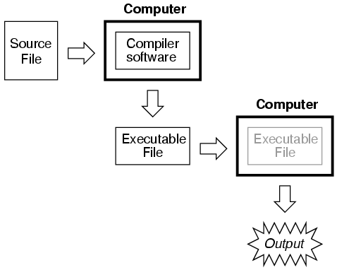
SPICE is an interpreted language. In order for a computer to be able to understand the SPICE instructions you type, it must have the SPICE program (interpreter) installed:

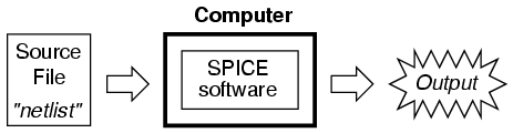
SPICE source files are commonly referred to as "netlists," although they are sometimes known as "decks" with each line in the file being called a "card." Cute, don't you think? Netlists are created by a person like yourself typing instructions line-by-line using a word processor or text editor. Text editors are much preferred over word processors for any type of computer programming, as they produce pure ASCII text with no special embedded codes for text highlighting (like italic or boldface fonts), which are uninterpretable by interpreter and compiler software.

As in general programming, the source file you create for SPICE must follow certain conventions of programming. It is a computer language in itself, albeit a simple one. Having programmed in BASIC and C/C++, and having some experience reading PASCAL and FORTRAN programs, it is my opinion that the language of SPICE is much simpler than any of these. It is about the same complexity as a markup language such as HTML, perhaps less so.

There is a cycle of steps to be followed in using SPICE to analyze a circuit. The cycle starts when you first invoke the text editing program and make your first draft of the netlist. The next step is to run SPICE on that new netlist and see what the results are. If you are a novice user of SPICE, your first attempts at creating a good netlist will be fraught with small errors of syntax. Don't worry -- as every computer programmer knows, proficiency comes with lots of practice. If your trial run produces error messages or results that are obviously incorrect, you need to re-invoke the text editing program and modify the netlist. After modifying the netlist, you need to run SPICE again and check the results. The sequence, then, looks something like this:

• Compose a new netlist with a text editing program. Save that netlist to a file with a name of your choice.
• Run SPICE on that netlist and observe the results.
• If the results contain errors, start up the text editing program again and modify the netlist.
• Run SPICE again and observe the new results.
• If there are still errors in the output of SPICE, re-edit the netlist again with the text editing program. Repeat this cycle of edit/run as many times as necessary until you are getting the desired results.
• Once you've "debugged" your netlist and are getting good results, run SPICE again, only this time redirecting the output to a new file instead of just observing it on the computer screen.
• Start up a text editing program or a word processor program and open the SPICE output file you just created. Modify that file to suit your formatting needs and either save those changes to disk and/or print them out on paper.

To "run" a SPICE "program," you need to type in a command at a terminal prompt interface, such as that found in MS-DOS, UNIX, or the MS-Windows DOS prompt option:

spice <>

The word "spice" invokes the SPICE interpreting program (providing that the SPICE software has been installed on the computer!), the "<" symbol redirects the contents of the source file to the SPICE interpreter, and example.cir is the name of the source file for this circuit example.  The file extension ".cir" is not mandatory; I have seen ".inp" (for "input") and just plain ".txt" work well, too. It will even work when the netlist file has no extension. SPICE doesn't care what you name it, so long as it has a name compatible with the filesystem of your computer (for old MS-DOS machines, for example, the filename must be no more than 8 characters in length, with a 3 character extension, and no spaces or other non-alphanumerical characters). 
  
 When this command is typed in, SPICE will read the contents of the example.cir file, analyze the circuit specified by that file, and send a text report to the computer terminal's standard output (usually the screen, where you can see it scroll by). A typical SPICE output is several screens worth of information, so you might want to look it over with a slight modification of the command: 

spice <>

This alternative "pipes" the text output of SPICE to the "more" utility, which allows only one page to be displayed at a time. What this means (in English) is that the text output of SPICE is halted after one screen-full, and waits until the user presses a keyboard key to display the next screen-full of text. If you're just testing your example circuit file and want to check for any errors, this is a good way to do it. 

spice <> example.txt


 This second alternative (above) redirects the text output of SPICE to another file, called example.txt, where it can be viewed or printed. This option corresponds to the last step in the development cycle listed earlier. It is recommended by this author that you use this technique of "redirection" to a text file only after you've proven your example circuit netlist to work well, so that you don't waste time invoking a text editor just to see the output during the stages of "debugging." 
  
 Once you have a SPICE output stored in a .txt file, you can use a text editor or (better yet!) a word processor to edit the output, deleting any unnecessary banners and messages, even specifying alternative fonts to highlight the headings and/or data for a more polished appearance. Then, of course, you can print the output to paper if you so desire. Being that the direct SPICE output is plain ASCII text, such a file will be universally interpretable on any computer whether SPICE is installed on it or not. Also, the plain text format ensures that the file will be very small compared to the graphic screen-shot files generated by "point-and-click" simulators. 
  
The netlist file format required by SPICE is quite simple. A netlist file is nothing more than a plain ASCII text file containing multiple lines of text, each line describing either a circuit component or special SPICE command. Circuit architecture is specified by assigning numbers to each component's connection points in each line, connections between components designated by common numbers. Examine the following example circuit diagram and its corresponding SPICE file. Please bear in mind that the circuit diagram exists only to make the simulation easier for human beings to understand. SPICE only understands netlists: 
  
  

Example netlist
v1 1 0 dc 15
r1 1 0 2.2k
r2 1 2 3.3k
r3 2 0 150
.end


 Each line of the source file shown above is explained here: 
  
v1 represents the battery (voltage source 1), positive terminal numbered 1, negative terminal numbered 0, with a DC voltage output of 15 volts.
r1 represents resistor R1 in the diagram, connected between points 1 and 0, with a value of 2.2 kΩ.
r2 represents resistor R2 in the diagram, connected between points 1 and 2, with a value of 3.3 kΩ.
r3 represents resistor R3 in the diagram, connected between points 2 and 0, with a value of 150 kΩ.
    
 Electrically common points (or "nodes") in a SPICE circuit description share common numbers, much in the same way that wires connecting common points in a large circuit typically share common wire labels. 
  
To simulate this circuit, the user would type those six lines of text on a text editor and save them as a file with a unique name (such as example.cir). Once the netlist is composed and saved to a file, the user then processes that file with one of the command-line statements shown earlier (spice <>), and will receive this text output on their computer's screen: 


1*******10/10/99 ******** spice 2g.6 3/15/83 ********07:32:42*****

0example netlist

0****   input listing                 temperature =   27.000 deg c

v1 1 0 dc 15
r1 1 0 2.2k
r2 1 2 3.3k
r3 2 0 150 
.end

*****10/10/99 *********  spice 2g.6  3/15/83 ******07:32:42******

0example netlist
0****   small signal bias solution     temperature =   27.000 deg c


node   voltage     node   voltage

(  1)   15.0000    (  2)    0.6522


voltage source currents
name       current

v1       -1.117E-02


total power dissipation   1.67E-01  watts

   job concluded
0         total job time            0.02
1*******10/10/99 ********  spice 2g.6  3/15/83 ******07:32:42*****


0****   input listing                 temperature =   27.000 deg c


 SPICE begins by printing the time, date, and version used at the top of the output. It then lists the input parameters (the lines of the source file), followed by a display of DC voltage readings from each node (reference number) to ground (always reference number 0). This is followed by a list of current readings through each voltage source (in this case there's only one, v1). Finally, the total power dissipation and computation time in seconds is printed. 
  
 All output values provided by SPICE are displayed in scientific notation. 
  
The SPICE output listing shown above is a little verbose for most peoples' taste. For a final presentation, it might be nice to trim all the unnecessary text and leave only what matters. Here is a sample of that same output, redirected to a text file (spice <> example.txt), then trimmed down judiciously with a text editor for final presentation and printed: 


example netlist
v1 1 0 dc 15
r1 1 0 2.2k
r2 1 2 3.3k
r3 2 0 150 
.end


node    voltage    node     voltage
(  1)   15.0000    (  2)    0.6522


voltage source currents
name       current
v1       -1.117E-02


total power dissipation   1.67E-01  watts


 One of the very nice things about SPICE is that both input and output formats are plain-text, which is the most universal and easy-to-edit electronic format around. Practically any computer will be able to edit and display this format, even if the SPICE program itself is not resident on that computer. If the user desires, he or she is free to use the advanced capabilities of word processing programs to make the output look fancier. Comments can even be inserted between lines of the output for further clarity to the reader. 
         
The command-line interface
  
If you've used DOS or UNIX operating systems before in a command-line shell environment, you may wonder why we have to use the "<" symbol between the word "spice" and the name of the netlist file to be interpreted. Why not just enter the file name as the first argument to the command "spice" as we do when we invoke the text editor? The answer is that SPICE has the option of an interactive mode, whereby each line of the netlist can be interpreted as it is entered through the computer's Standard Input (stdin). If you simple type "spice" at the prompt and press [Enter], SPICE will begin to interpret anything you type in to it (live). 
  
 For most applications, its nice to save your netlist work in a separate file and then let SPICE interpret that file when you're ready. This is the way I encourage SPICE to be used, and so this is the way its presented in this lesson. In order to use SPICE this way in a command-line environment, we need to use the "<" redirection symbol to direct the contents of your netlist file to Standard Input (stdin), which SPICE can then process. 
         
Circuit components
  
Remember that this tutorial is not exhaustive by any means, and that all descriptions for elements in the SPICE language are documented here in condensed form. SPICE is a very capable piece of software with lots of options, and I'm only going to document a few of them. 
  
 All components in a SPICE source file are primarily identified by the first letter in each respective line. Characters following the identifying letter are used to distinguish one component of a certain type from another of the same type (r1, r2, r3, rload, rpullup, etc.), and need not follow any particular naming convention, so long as no more than eight characters are used in both the component identifying letter and the distinguishing name. 
    
 For example, suppose you were simulating a digital circuit with "pullup" and "pulldown" resistors.  The name rpullup would be valid because it is seven characters long.  The name rpulldown, however, is nine characters long.  This may cause problems when SPICE interprets the netlist. 
  
 You can actually get away with component names in excess of eight total characters if there are no other similarly-named components in the source file. SPICE only pays attention to the first eight characters of the first field in each line, so rpulldown is actually interpreted as rpulldow with the "n" at the end being ignored. Therefore, any other resistor having the first eight characters in its first field will be seen by SPICE as the same resistor, defined twice, which will cause an error (i.e. rpulldown1 and rpulldown2 would be interpreted as the same name, rpulldow). 
  
 It should also be noted that SPICE ignores character case, so r1 and R1 are interpreted by SPICE as one and the same. 
  
 SPICE allows the use of metric prefixes in specifying component values, which is a very handy feature. However, the prefix convention used by SPICE differs somewhat from standard metric symbols, primarily due to the fact that netlists are restricted to standard ASCII characters (ruling out Greek letters such as µ for the prefix "micro") and that SPICE is case-insensitive, so "m" (which is the standard symbol for "milli") and "M" (which is the standard symbol for "Mega") are interpreted identically. Here are a few examples of prefixes used in SPICE netlists: 
  

 r1 1 0 2t (Resistor R1, 2t = 2 Tera-ohms = 2 TΩ) 
  
 r2 1 0 4g (Resistor R2, 4g = 4 Giga-ohms = 4 GΩ) 
  
 r3 1 0 47meg (Resistor R3, 47meg = 47 Mega-ohms = 47 MΩ) 
  
 r4 1 0 3.3k (Resistor R4, 3.3k = 3.3 kilo-ohms = 3.3 kΩ) 
  
 r5 1 0 55m (Resistor R5, 55m = 55 milli-ohms = 55 mΩ) 
  
 r6 1 0 10u (Resistor R6, 10u = 10 micro-ohms 10 µΩ) 
  
 r7 1 0 30n (Resistor R7, 30n = 30 nano-ohms = 30 nΩ) 
  
 r8 1 0 5p (Resistor R8, 5p = 5 pico-ohms = 5 pΩ) 
  
 r9 1 0 250f (Resistor R9, 250f = 250 femto-ohms = 250 fΩ) 


  
 Scientific notation is also allowed in specifying component values.  For example: 


 r10 1 0 4.7e3 (Resistor R10, 4.7e3 = 4.7 x 103 ohms = 4.7 kilo-ohms = 4.7 kΩ) 
  
 r11 1 0 1e-12 (Resistor R11, 1e-12 = 1 x 10-12 ohms = 1 pico-ohm = 1 pΩ) 


The unit (ohms, volts, farads, henrys, etc.) is automatically determined by the type of component being specified. SPICE "knows" that all of the above examples are "ohms" because they are all resistors (r1, r2, r3, . . . ). If they were capacitors, the values would be interpreted as "farads," if inductors, then "henrys," etc. 
     
Passive components
   
CAPACITORS
   
General form:  c[name] [node1] [node2] [value] ic=[initial voltage]
Example 1:     c1 12 33 10u
Example 2:     c1 12 33 10u ic=3.5

  
 Comments:  The "initial condition" (ic=) variable is the capacitor's voltage in units of volts at the start of DC analysis. It is an optional value, with the starting voltage assumed to be zero if unspecified. Starting current values for capacitors are interpreted by SPICE only if the .tran analysis option is invoked (with the "uic" option).  
      
INDUCTORS
   
General form:  l[name] [node1] [node2] [value] ic=[initial current]
Example 1:     l1 12 33 133m
Example 2:     l1 12 33 133m ic=12.7m

  
 Comments:  The "initial condition" (ic=) variable is the inductor's current in units of amps at the start of DC analysis. It is an optional value, with the starting current assumed to be zero if unspecified. Starting current values for inductors are interpreted by SPICE only if the .tran analysis option is invoked. 
     
INDUCTOR COUPLING (transformers)
    
General form:  k[name] l[name] l[name] [coupling factor]
Example 1:     k1 l1 l2 0.999

  
 Comments: SPICE will only allow coupling factor values between 0 and 1 (non-inclusive), with 0 representing no coupling and 1 representing perfect coupling. The order of specifying coupled inductors (l1, l2 or l2, l1) is irrelevant. 
      
RESISTORS
    
General form:  r[name] [node1] [node2] [value]
Example:       rload 23 15 3.3k

  
 Comments: In case you were wondering, there is no declaration of resistor power dissipation rating in SPICE. All components are assumed to be indestructible. If only real life were this forgiving! 
           
Active components
     
 All semiconductor components must have their electrical characteristics described in a line starting with the word ".model", which tells SPICE exactly how the device will behave.  Whatever parameters are not explicitly defined in the .model card will default to values pre-programmed in SPICE.  However, the .model card must be included, and at least specify the model name and device type (d, npn, pnp, njf, pjf, nmos, or pmos). 
   
DIODES
    
General form:  d[name] [anode] [cathode] [model]
Example:       d1 1 2 mod1

  
 DIODE MODELS: 
  
General form:  .model [modelname] d [parmtr1=x] [parmtr2=x] . . .
Example:       .model mod1 d
Example:       .model mod2 d vj=0.65 rs=1.3

  diodeparameter  
 Parameter definitions: 
  
 is = saturation current in amps 
  
 rs = junction resistance in ohms 
  
 n = emission coefficient (unitless) 
  
 tt = transit time in seconds 
  
 cjo = zero-bias junction capacitance in farads 
  
 vj = junction potential in volts 
  
 m = grading coefficient (unitless) 
  
 eg = activation energy in electron-volts 
  
 xti = saturation-current temperature exponent (unitless) 
  
 kf = flicker noise coefficient (unitless) 
  
 af = flicker noise exponent (unitless) 
  
 fc = forward-bias depletion capacitance coefficient (unitless) 
  
 bv = reverse breakdown voltage in volts 
  
 ibv = current at breakdown voltage in amps 


 Comments:  The model name must begin with a letter, not a number. If you plan to specify a model for a 1N4003 rectifying diode, for instance, you cannot use "1n4003" for the model name. An alternative might be "m1n4003" instead. 
     
TRANSISTORS, bipolar junction -- BJT
   
General form:  q[name] [collector] [base] [emitter] [model]
Example:       q1 2 3 0 mod1

  
 BJT TRANSISTOR MODELS: 
  
General form:  .model [modelname] [npn or pnp] [parmtr1=x] . . .
Example:       .model mod1 pnp
Example:       .model mod2 npn bf=75 is=1e-14

  
The model examples shown above are very nonspecific. To accurately model real-life transistors, more parameters are necessary. Take these two examples, for the popular 2N2222 and 2N2907 transistors (the "+") characters represent line-continuation marks in SPICE, when you wish to break a single line (card) into two or more separate lines on your text editor: 
  

Example:       .model m2n2222 npn is=19f bf=150 vaf=100 ikf=.18
+                     ise=50p ne=2.5 br=7.5 var=6.4 ikr=12m
+                     isc=8.7p nc=1.2 rb=50 re=0.4 rc=0.4 cje=26p
+                     tf=0.5n cjc=11p tr=7n xtb=1.5 kf=0.032f af=1

  
Example:       .model m2n2907 pnp is=1.1p bf=200 nf=1.2 vaf=50
+                     ikf=0.1 ise=13p ne=1.9 br=6 rc=0.6 cje=23p
+                     vje=0.85 mje=1.25 tf=0.5n cjc=19p vjc=0.5
+                     mjc=0.2 tr=34n xtb=1.5

  
 Parameter definitions: 
  
 is = transport saturation current in amps 
  
 bf = ideal maximum forward Beta (unitless) 
  
 nf = forward current emission coefficient (unitless) 
  
 vaf = forward Early voltage in volts 
  
 ikf = corner for forward Beta high-current rolloff in amps 
  
 ise = B-E leakage saturation current in amps 
  
 ne = B-E leakage emission coefficient (unitless) 
  
 br = ideal maximum reverse Beta (unitless) 
  
 nr = reverse current emission coefficient (unitless) 
  
 bar = reverse Early voltage in volts 
  
 ikrikr = corner for reverse Beta high-current rolloff in amps 
  
 iscisc = B-C leakage saturation current in amps 
  
 nc = B-C leakage emission coefficient (unitless) 
  
 rb = zero bias base resistance in ohms 
  
 irb = current for base resistance halfway value in amps 
  
 rbm = minimum base resistance at high currents in ohms 
  
 re = emitter resistance in ohms 
  
 rc = collector resistance in ohms 
  
 cje = B-E zero-bias depletion capacitance in farads 
  
 vje = B-E built-in potential in volts 
  
 mje = B-E junction exponential factor (unitless) 
  
 tf = ideal forward transit time (seconds) 
  
 xtf = coefficient for bias dependence of transit time (unitless) 
  
 vtf = B-C voltage dependence on transit time, in volts 
  
 itf = high-current parameter effect on transit time, in amps 
  
 ptf = excess phase at f=1/(transit time)(2)(pi) Hz, in degrees 
  
 cjc = B-C zero-bias depletion capacitance in farads 
  
 vjc = B-C built-in potential in volts 
  
 mjc = B-C junction exponential factor (unitless) 
  
 xjcj = B-C depletion capacitance fraction connected in base node (unitless) 
  
 tr = ideal reverse transit time in seconds 
  
 cjs = zero-bias collector-substrate capacitance in farads 
  
 vjs = substrate junction built-in potential in volts 
  
 mjs = substrate junction exponential factor (unitless) 
  
 xtb = forward/reverse Beta temperature exponent 
  
 eg = energy gap for temperature effect on transport saturation current in electron-volts 
  
 xti = temperature exponent for effect on transport saturation current (unitless) 
  
 kf = flicker noise coefficient (unitless) 
  
 af = flicker noise exponent (unitless) 
  
 fc = forward-bias depletion capacitance formula coefficient (unitless) 


 Comments:  Just as with diodes, the model name given for a particular transistor type must begin with a letter, not a number. That's why the examples given above for the 2N2222 and 2N2907 types of BJTs are named "m2n2222" and "q2n2907" respectively. 
  
As you can see, SPICE allows for very detailed specification of transistor properties. Many of the properties listed above are well beyond the scope and interest of the beginning electronics student, and aren't even useful apart from knowing the equations SPICE uses to model BJT transistors. For those interested in learning more about transistor modeling in SPICE, consult other books, such as Andrei Vladimirescu's The Spice Book (ISBN 0-471-60926-9). 
      
JFET, junction field-effect transistor
   
General form:  j[name] [drain] [gate] [source] [model]
Example:       j1 2 3 0 mod1

  
 JFET TRANSISTOR MODELS: 
  
General form:     .model [modelname] [njf or pjf] [parmtr1=x] . . .
Example:          .model mod1 pjf
Example:          .model mod2 njf lambda=1e-5 pb=0.75

  
 Parameter definitions: 
  
 vto = threshold voltage in volts 
  
 beta = transconductance parameter in amps/volts2 
  
 lambda = channel length modulation parameter in units of 1/volts 
  
 rd = drain resistance in ohms 
  
 rs = source resistance in ohms 
  
 cgs = zero-bias G-S junction capacitance in farads 
  
 cgd = zero-bias G-D junction capacitance in farads 
  
 pb = gate junction potential in volts 
  
 is = gate junction saturation current in amps 
  
 kf = flicker noise coefficient (unitless) 
  
 af = flicker noise exponent (unitless) 
  
 fc = forward-bias depletion capacitance coefficient (unitless) 
     
MOSFET, transistor
   
General form:  m[name] [drain] [gate] [source] [substrate] [model]
Example:       m1 2 3 0 0 mod1

  
 MOSFET TRANSISTOR MODELS: 
  
General form:  .model [modelname] [nmos or pmos] [parmtr1=x] . . .
Example:       .model mod1 pmos
Example:       .model mod2 nmos level=2 phi=0.65 rd=1.5
Example:       .model mod3 nmos vto=-1   (depletion)
Example:       .model mod4 nmos vto=1    (enhancement)
Example:       .model mod5 pmos vto=1    (depletion)
Example:       .model mod6 pmos vto=-1   (enhancement)

  
 Comments: In order to distinguish between enhancement mode and depletion-mode (also known as depletion-enhancement mode) transistors, the model parameter "vto" (zero-bias threshold voltage) must be specified. Its default value is zero, but a positive value (+1 volts, for example) on a P-channel transistor or a negative value (-1 volts) on an N-channel transistor will specify that transistor to be a depletion (otherwise known as depletion-enhancement) mode device. Conversely, a negative value on a P-channel transistor or a positive value on an N-channel transistor will specify that transistor to be an enhancement mode device. 
  
 Remember that enhancement mode transistors are normally-off devices, and must be turned on by the application of gate voltage. Depletion-mode transistors are normally "on," but can be "pinched off" as well as enhanced to greater levels of drain current by applied gate voltage, hence the alternate designation of "depletion-enhancement" MOSFETs. The "vto" parameter specifies the threshold gate voltage for MOSFET conduction. 
         
Sources
    
 AC SINEWAVE VOLTAGE SOURCES (when using .ac card to specify frequency): 
  
General form:  v[name] [+node] [-node] ac [voltage] [phase] sin
Example 1:     v1 1 0 ac 12 sin
Example 2:     v1 1 0 ac 12 240 sin   (12 V ∠ 240o)
  
 Comments: This method of specifying AC voltage sources works well if you're using multiple sources at different phase angles from each other, but all at the same frequency. If you need to specify sources at different frequencies in the same circuit, you must use the next method! 


 AC SINEWAVE VOLTAGE SOURCES (when NOT using .ac card to specify frequency): 
  
General form:  v[name] [+node] [-node] sin([offset] [voltage]
+               [freq] [delay] [damping factor])
Example 1:     v1 1 0 sin(0 12 60 0 0)
  
 Parameter definitions: 
  
 offset = DC bias voltage, offsetting the AC waveform by a specified voltage. 
  
 voltage = peak, or crest, AC voltage value for the waveform. 
  
 freq = frequency in Hertz. 
  
 delay = time delay, or phase offset for the waveform, in seconds. 
  
 damping factor = a figure used to create waveforms of decaying amplitude. 
  
 Comments: This method of specifying AC voltage sources works well if you're using multiple sources at different frequencies from each other. Representing phase shift is tricky, though, necessitating the use of the delay factor.  


  
 DC VOLTAGE SOURCES (when using .dc card to specify voltage): 
  
General form:  v[name] [+node] [-node] dc
Example 1:     v1 1 0 dc
  
 Comments: If you wish to have SPICE output voltages not in reference to node 0, you must use the .dc analysis option, and to use this option you must specify at least one of your DC sources in this manner. 


 DC VOLTAGE SOURCES (when NOT using .dc card to specify voltage): 
  
General form:  v[name] [+node] [-node] dc [voltage]
Example 1:     v1 1 0 dc 12
  
 Comments: Nothing noteworthy here!  


  
 PULSE VOLTAGE SOURCES 
  
General form:  v[name] [+node] [-node] pulse ([i] [p] [td] [tr]
+              [tf] [pw] [pd])
  
 Parameter definitions: 
  
 i = initial value 
  
 p = pulse value 
  
 td = delay time (all time parameters in units of seconds) 
  
 tr = rise time 
  
 tf = fall time 
  
 pw = pulse width 
  
 pd = period 
  
Example 1:     v1 1 0 pulse (-3 3 0 0 0 10m 20m)
  
 Comments: Example 1 is a perfect square wave oscillating between -3 and +3 volts, with zero rise and fall times, a 20 millisecond period, and a 50 percent duty cycle (+3 volts for 10 ms, then -3 volts for 10 ms). 


  
 AC SINEWAVE CURRENT SOURCES (when using .ac card to specify frequency): 
  
General form:  i[name] [+node] [-node] ac [current] [phase] sin
Example 1:     i1 1 0 ac 3 sin        (3 amps)
Example 2:     i1 1 0 ac 1m 240 sin   (1 mA ∠ 240o)
  
 Comments:  The same comments apply here (and in the next example) as for AC voltage sources. 


 AC SINEWAVE CURRENT SOURCES (when NOT using .ac card to specify frequency): 
  
General form:  i[name] [+node] [-node] sin([offset]
+              [current] [freq] 0 0)
Example 1:     i1 1 0 sin(0 1.5 60 0 0)


  
 DC CURRENT SOURCES (when using .dc card to specify current): 
  
General form:  i[name] [+node] [-node] dc
Example 1:     i1 1 0 dc


 DC CURRENT SOURCES (when NOT using .dc card to specify current): 
  
General form:  i[name] [+node] [-node] dc [current]
Example 1:     i1 1 0 dc 12
  
 Comments: Even though the books all say that the first node given for the DC current source is the positive node, that's not what I've found to be in practice. In actuality, a DC current source in SPICE pushes current in the same direction as a voltage source (battery) would with its negative node specified first. 


  
 PULSE CURRENT SOURCES 
  
General form:  i[name] [+node] [-node] pulse ([i] [p] [td] [tr]
+              [tf] [pw] [pd])
  
 Parameter definitions: 
  
 i = initial value 
  
 p = pulse value 
  
 td = delay time 
  
 tr = rise time 
  
 tf = fall time 
  
 pw = pulse width 
  
 pd = period 
  
Example 1:     i1 1 0 pulse (-3m 3m 0 0 0 17m 34m)
  
 Comments: Example 1 is a perfect square wave oscillating between -3 mA and +3 mA, with zero rise and fall times, a 34 millisecond period, and a 50 percent duty cycle (+3 mA for 17 ms, then -3 mA for 17 ms). 


  
 VOLTAGE SOURCES (dependent): 
  
General form:  e[name] [out+node] [out-node] [in+node] [in-node]
+               [gain]
Example 1:     e1 2 0 1 2 999k
  
 Comments: Dependent voltage sources are great to use for simulating operational amplifiers. Example 1 shows how such a source would be configured for use as a voltage follower, inverting input connected to output (node 2) for negative feedback, and the noninverting input coming in on node 1. The gain has been set to an arbitrarily high value of 999,000. One word of caution, though: SPICE does not recognize the input of a dependent source as being a load, so a voltage source tied only to the input of an independent voltage source will be interpreted as "open." See op-amp circuit examples for more details on this. 


  
 CURRENT SOURCES (dependent): 
           
Analysis options
    
 AC ANALYSIS: 
  
General form:  .ac [curve] [points] [start] [final]
Example 1:     .ac lin 1 1000 1000
  
 Comments: The [curve] field can be "lin" (linear), "dec" (decade), or "oct" (octave), specifying the (non)linearity of the frequency sweep.  specifies how many points within the frequency sweep to perform analyses at (for decade sweep, the number of points per decade; for octave, the number of points per octave). The [start] and [final] fields specify the starting and ending frequencies of the sweep, respectively. One final note: the "start" value cannot be zero! 


  
 DC ANALYSIS: 
  
General form:     .dc [source] [start] [final] [increment]
Example 1:        .dc vin 1.5 15 0.5
  
 Comments: The .dc card is necessary if you want to print or plot any voltage between two nonzero nodes. Otherwise, the default "small-signal" analysis only prints out the voltage between each nonzero node and node zero. 


  
 TRANSIENT ANALYSIS: 
  
General form:  .tran [increment] [stop_time] [start_time]
+                    [comp_interval]
Example 1:     .tran 1m 50m uic
Example 2:     .tran .5m 32m 0 .01m
  
 Comments: Example 1 has an increment time of 1 millisecond and a stop time of 50 milliseconds (when only two parameters are specified, they are increment time and stop time, respectively). Example 2 has an increment time of 0.5 milliseconds, a stop time of 32 milliseconds, a start time of 0 milliseconds (no delay on start), and a computation interval of 0.01 milliseconds. 
  
 Default value for start time is zero.  Transient analysis always beings at time zero, but storage of data only takes place between start time and stop time. Data output interval is increment time, or (stop time - start time)/50, which ever is smallest. However, the computing interval variable can be used to force a computational interval smaller than either. For large total interval counts, the itl5 variable in the .options card may be set to a higher number.  The "uic" option tells SPICE to "use initial conditions." 


  
 PLOT OUTPUT: 
  
General form:  .plot [type] [output1] [output2] . . . [output n]
Example 1:     .plot dc v(1,2) i(v2)
Example 2:     .plot ac v(3,4) vp(3,4) i(v1) ip(v1)
Example 3:     .plot tran v(4,5) i(v2)
  
 Comments:  SPICE can't handle more than eight data point requests on a single .plot or .print card.  If requesting more than eight data points, use multiple cards! 
  
 Also, here's a major caveat when using SPICE version 3: if you're performing AC analysis and you ask SPICE to plot an AC voltage as in example #2, the v(3,4) command will only output the real component of a rectangular-form complex number!  SPICE version 2 outputs the polar magnitude of a complex number: a much more meaningful quantity if only a single quantity is asked for. To coerce SPICE3 to give you polar magnitude, you will have to re-write the .print or .plot argument as such: vm(3,4). 


  
 PRINT OUTPUT: 
  
General form:  .print [type] [output1] [output2] . . . [output n]
Example 1:     .print dc v(1,2) i(v2)
Example 2:     .print ac v(2,4) i(vinput) vp(2,3)
Example 3:     .print tran v(4,5) i(v2)
  
 Comments:  SPICE can't handle more than eight data point requests on a single .plot or .print card.  If requesting more than eight data points, use multiple cards! 


  
 FOURIER ANALYSIS: 
  
General form:  .four [freq] [output1] [output2] . . . [output n]
Example 1:     .four 60 v(1,2)
  
 Comments:  The .four card relies on the .tran card being present somewhere in the deck, with the proper time periods for analysis of adequate cycles. Also, SPICE may "crash" if a .plot analysis isn't done along with the .four analysis, even if all .tran parameters are technically correct.  Finally, the .four analysis option only works when the frequency of the AC source is specified in that source's card line, and not in an .ac analysis option line. 
  
 It helps to include a computation interval variable in the .tran card for better analysis precision. A Fourier analysis of the voltage or current specified is performed up to the 9th harmonic, with the [freq] specification being the fundamental, or starting frequency of the analysis spectrum. 


  
 MISCELLANEOUS: 
  
General form:  .options [option1] [option2]
Example 1:     .options limpts=500
Example 2:     .options itl5=0
Example 3:     .options method=gear
Example 4:     .options list
Example 5:     .options nopage
Example 6:     .options numdgt=6
  limpts, SPICE">  
 Comments: There are lots of options that can be specified using this card. Perhaps the one most needed by beginning users of SPICE is the "limpts" setting. When running a simulation that requires more than 201 points to be printed or plotted, this calculation point limit must be increased or else SPICE will terminate analysis. The example given above (limpts=500) tells SPICE to allocate enough memory to handle at least 500 calculation points in whatever type of analysis is specified (DC, AC, or transient). 
  itl5, SPICE">  
 In example 2, we see an iteration variable (itl5) being set to a value of 0. There are actually six different iteration variables available for user manipulation. They control the iteration cycle limits for solution of nonlinear equations. The variable itl5 sets the maximum number of iterations for a transient analysis.  Similar to the limpts variable, itl5 usually needs to be set when a small computation interval has been specified on a .tran card.  Setting itl5 to a value of 0 turns off the limit entirely, allowing the computer infinite iteration cycles (infinite time) to compute the analysis. Warning: this may result in long simulation times! 
  method, SPICE">  
 Example 3 with "method=gear" sets the numerical integration method used by SPICE. The default is "trapezoid" rather than "gear," trapezoid being a simple geometric approximation of area under a curve found by slicing up the curve into trapezoids to approximate the shape. The "gear" method is based on second-order or better polynomial equations and is named after C.W. Gear (Numerical Integration of Stiff Ordinary Equations, Report 221, Department of Computer Science, University of Illinois, Urbana). The Gear method of integration is more demanding of the computer (computationally "expensive") and will sometimes give slightly different results from the trapezoid method. 
  list, SPICE">  
 The "list" option shown in example 4 gives a verbose summary of all circuit components and their respective values in the final output. 
  nopage, SPICE">  
By default, SPICE will insert ASCII page-break control codes in the output to separate different sections of the analysis. Specifying the "nopage" option (example 5) will prevent such pagination. 
  numdgt, SPICE">  
 The "numdgt" option shown in example 6 specifies the number of significant digits output when using one of the ".print" data output options.  SPICE defaults at a precision of 4 significant digits. 


 WIDTH CONTROL: 
  
General form:  .width in=[columns] out=[columns]
Example 1:     .width out=80
  width, SPICE">  
 Comments:  The .width card can be used to control the width of text output lines upon analysis. This is especially handy when plotting graphs with the .plot card. The default value is 120, which can cause problems on 80-character terminal displays unless set to 80 with this command. 
          
Quirks
  
  
 "Garbage in, garbage out." 
  
 Anonymous 
  
  
 SPICE is a very reliable piece of software, but it does have its little quirks that take some getting used to. By "quirk" I mean a demand placed upon the user to write the source file in a particular way in order for it to work without giving error messages. I do not mean any kind of fault with SPICE which would produce erroneous or misleading results: that would be more properly referred to as a "bug." Speaking of bugs, SPICE has a few of them as well. 
  
Some (or all) of these quirks may be unique to SPICE version 2g6, which is the only version I've used extensively. They may have been fixed in later versions. 
     
A good beginning
  
SPICE demands that the source file begin with something other than the first "card" in the circuit description "deck." This first character in the source file can be a linefeed, title line, or a comment: there just has to be something there before the first component-specifying line of the file. If not, SPICE will refuse to do an analysis at all, claiming that there is a serious error (such as improper node connections) in the "deck." 
       
A good ending
    
 SPICE demands that the .end line at the end of the source file not be terminated with a linefeed or carriage return character. In other words, when you finish typing ".end" you should not hit the [Enter] key on your keyboard.  The cursor on your text editor should stop immediately to the right of the "d" after the ".end" and go no further.  Failure to heed this quirk will result in a "missing .end card" error message at the end of the analysis output. The actual circuit analysis is not affected by this error, so I normally ignore the message. However, if you're looking to receive a "perfect" output, you must pay heed to this idiosyncrasy. 
       
Must have a node 0
    
 You are given much freedom in numbering circuit nodes, but you must have a node 0 somewhere in your netlist in order for SPICE to work. Node 0 is the default node for circuit ground, and it is the point of reference for all voltages specified at single node locations. 
  
When simple DC analysis is performed by SPICE, the output will contain a listing of voltages at all non-zero nodes in the circuit. The point of reference (ground) for all these voltage readings is node 0. For example: 


node    voltage    node     voltage
(  1)   15.0000    (  2)    0.6522


In this analysis, there is a DC voltage of 15 volts between node 1 and ground (node 0), and a DC voltage of 0.6522 volts between node 2 and ground (node 0). In both these cases, the voltage polarity is negative at node 0 with reference to the other node (in other words, both nodes 1 and 2 are positive with respect to node 0). 
        
Avoid open circuits
    
SPICE cannot handle open circuits of any kind. If your netlist specifies a circuit with an open voltage source, for example, SPICE will refuse to perform an analysis. A prime example of this type of error is found when "connecting" a voltage source to the input of a voltage-dependent source (used to simulate an operational amplifier). SPICE needs to see a complete path for current, so I usually tie a high-value resistor (call it rbogus!) across the voltage source to act as a minimal load. 
       
Avoid certain component loops
  
 SPICE cannot handle certain uninterrupted loops of components in a circuit, namely voltage sources and inductors. The following loops will cause SPICE to abort analysis: 
  
  
   
netlist
l1 2 4 10m
l2 2 4 50m
l3 2 4 25m


  
   
netlist
v1 1 0 dc 12
l1 1 0 150m


  
   
netlist
c1 5 6 33u
c2 6 7 47u


The reason SPICE can't handle these conditions stems from the way it performs DC analysis: by treating all inductors as shorts and all capacitors as opens. Since short-circuits (0 Ω) and open circuits (infinite resistance) either contain or generate mathematical infinitudes, a computer simply cannot deal with them, and so SPICE will discontinue analysis if any of these conditions occur. 
  
In order to make these component configurations acceptable to SPICE, you must insert resistors of appropriate values into the appropriate places, eliminating the respective short-circuits and open-circuits. If a series resistor is required, choose a very low resistance value. Conversely, if a parallel resistor is required, choose a very high resistance value. For example: 
  
 To fix the parallel inductor problem, insert a very low-value resistor in series with each offending inductor. 
  
  
   
original netlist
l1 2 4 10m
l2 2 4 50m
l3 2 4 25m


fixed netlist
rbogus1 2 3 1e-12
rbogus2 2 5 1e-12
l1 3 4 10m
l2 2 4 50m
l3 5 4 25m


 The extremely low-resistance resistors Rbogus1 and Rbogus2 (each one with a mere 1 pico-ohm of resistance) "break up" the direct parallel connections that existed between L1, L2, and L3.  It is important to choose very low resistances here so that circuit operation is not substantially impacted by the "fix." 
  
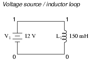
 To fix the voltage source / inductor loop, insert a very low-value resistor in series with the two components. 
  
  
   
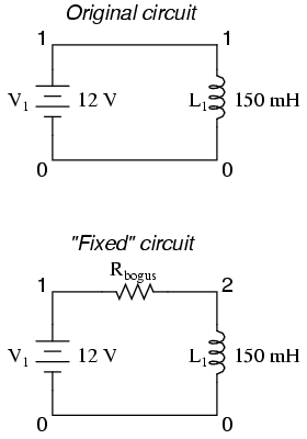
original netlist
v1 1 0 dc 12
l1 1 0 150m


fixed netlist
v1 1 0 dc 12
l1 2 0 150m
rbogus 1 2 1e-12


 As in the previous example with parallel inductors, it is important to make the correction resistor (Rbogus) very low in resistance, so as to not substantially impact circuit operation. 
  
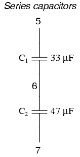
To fix the series capacitor circuit, one of the capacitors must have a resistor shunting across it. SPICE requires a DC current path to each capacitor for analysis. 
  
  
   
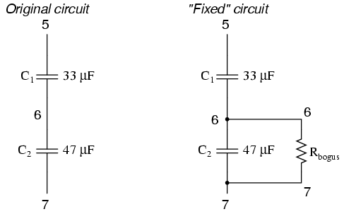
original netlist
c1 5 6 33u
c2 6 7 47u


fixed netlist
c1 5 6 33u
c2 6 7 47u
rbogus 6 7 9e12


 The Rbogus value of 9 Tera-ohms provides a DC current path to C1 (and around C2) without substantially impacting the circuit's operation. 
        
Current measurement
    
Although printing or plotting of voltage is quite easy in SPICE, the output of current values is a bit more difficult. Voltage measurements are specified by declaring the appropriate circuit nodes. For example, if we desire to know the voltage across a capacitor whose leads connect between nodes 4 and 7, we might make out .print statement look like this: 
  
  
   
c1 4 7 22u
.print ac v(4,7)


 However, if we wanted to have SPICE measure the current through that capacitor, it wouldn't be quite so easy. Currents in SPICE must be specified in relation to a voltage source, not any arbitrary component. For example: 
  
  
   
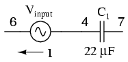
c1 4 7 22u
vinput 6 4 ac 1 sin
.print ac i(vinput)


 This .print card instructs SPICE to print the current through voltage source Vinput, which happens to be the same as the current through our capacitor between nodes 4 and 7. But what if there is no such voltage source in our circuit to reference for current measurement? One solution is to insert a shunt resistor into the circuit and measure voltage across it. In this case, I have chosen a shunt resistance value of 1 Ω to produce 1 volt per amp of current through C1: 
  
  
   
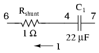
c1 4 7 22u
rshunt 6 4 1
.print ac v(6,4)


 However, the insertion of an extra resistance into our circuit large enough to drop a meaningful voltage for the intended range of current might adversely affect things. A better solution for SPICE is this, although one would never seek such a current measurement solution in real life: 
  
  
   
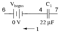
c1 4 7 22u
vbogus 6 4 dc 0
.print ac i(vbogus)


Inserting a "bogus" DC voltage source of zero volts doesn't affect circuit operation at all, yet it provides a convenient place for SPICE to take a current measurement. Interestingly enough, it doesn't matter that Vbogus is a DC source when we're looking to measure AC current! The fact that SPICE will output an AC current reading is determined by the "ac" specification in the .print card and nothing more. 
  
 It should also be noted that the way SPICE assigns a polarity to current measurements is a bit odd. Take the following circuit as an example: 
  
  
   
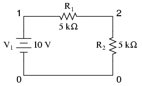
example
v1 1 0
r1 1 2 5k
r2 2 0 5k
.dc v1 10 10 1
.print dc i(v1)
.end


With 10 volts total voltage and 10 kΩ total resistance, you might expect SPICE to tell you there's going to be 1 mA (1e-03) of current through voltage source V1, but in actuality SPICE will output a figure of negative 1 mA (-1e-03)! SPICE regards current out of the negative end of a DC voltage source (the normal direction) to be a negative value of current rather than a positive value of current. There are times I'll throw in a "bogus" voltage source in a DC circuit like this simply to get SPICE to output a positive current value: 
  
  
   
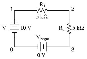
example
v1 1 0 
r1 1 2 5k
r2 2 3 5k   
vbogus 3 0 dc 0
.dc v1 10 10 1
.print dc i(vbogus)
.end


 Notice how Vbogus is positioned so that the circuit current will enter its positive side (node 3) and exit its negative side (node 0). This orientation will ensure a positive output figure for circuit current. 
        
Fourier analysis
    
When performing a Fourier (frequency-domain) analysis on a waveform, I have found it necessary to either print or plot the waveform using the .print or .plot cards, respectively. If you don't print or plot it, SPICE will pause for a moment during analysis and then abort the job after outputting the "initial transient solution." 
  
 Also, when analyzing a square wave produced by the "pulse" source function, you must give the waveform some finite rise and fall time, or else the Fourier analysis results will be incorrect. For some reason, a perfect square wave with zero rise/fall time produces significant levels of even harmonics according to SPICE's Fourier analysis option, which is not true for real square waves. 
           
Example circuits and netlists
  
 The following circuits are pre-tested netlists for SPICE 2g6, complete with short descriptions when necessary. Feel free to "copy" and "paste" any of the netlists to your own SPICE source file for analysis and/or modification. My goal here is twofold: to give practical examples of SPICE netlist design to further understanding of SPICE netlist syntax, and to show how simple and compact SPICE netlists can be in analyzing simple circuits. 
  
All output listings for these examples have been "trimmed" of extraneous information, giving you the most succinct presentation of the SPICE output as possible. I do this primarily to save space on this document. Typical SPICE outputs contain lots of headers and summary information not necessarily germane to the task at hand. So don't be surprised when you run a simulation on your own and find that the output doesn't exactly look like what I have shown here! 
      
Multiple-source DC resistor network, part 1
  
  
   
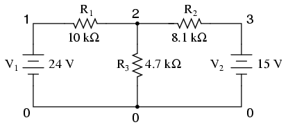
 Without a .dc card and a .print or .plot card, the output for this netlist will only display voltages for nodes 1, 2, and 3 (with reference to node 0, of course). 


 Netlist: 
  
Multiple dc sources
v1 1 0 dc 24
v2 3 0 dc 15
r1 1 2 10k
r2 2 3 8.1k
r3 2 0 4.7k
.end


 Output: 
  
node    voltage    node     voltage   node    voltage
(  1)   24.0000    (  2)    9.7470    (  3)   15.0000


voltage source currents
name       current
v1       -1.425E-03
v2       -6.485E-04


total power dissipation   4.39E-02  watts
        
Multiple-source DC resistor network, part 2
  
  
   
 By adding a .dc analysis card and specifying source V1 from 24 volts to 24 volts in 1 step (in other words, 24 volts steady), we can use the .print card analysis to print out voltages between any two points we desire.  Oddly enough, when the .dc analysis option is invoked, the default voltage printouts for each node (to ground) disappears, so we end up having to explicitly specify them in the .print card to see them at all. 


 Netlist: 
  
Multiple dc sources
v1 1 0
v2 3 0 15
r1 1 2 10k
r2 2 3 8.1k
r3 2 0 4.7k
.dc v1 24 24 1
.print dc v(1) v(2) v(3) v(1,2) v(2,3)
.end


 Output: 
  
v1           v(1)        v(2)        v(3)        v(1,2)      v(2,3)
2.400E+01    2.400E+01   9.747E+00   1.500E+01   1.425E+01  -5.253E+00
         
RC time-constant circuit
  
  
   
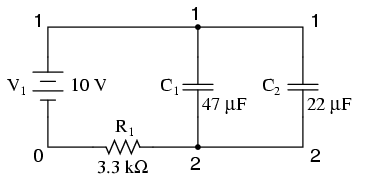
 For DC analysis, the initial conditions of any reactive component (C or L) must be specified (voltage for capacitors, current for inductors). This is provided by the last data field of each capacitor card (ic=0).  To perform a DC analysis, the .tran ("transient") analysis option must be specified, with the first data field specifying time increment in seconds, the second specifying total analysis timespan in seconds, and the "uic" telling it to "use initial conditions" when analyzing. 


 Netlist: 
  
RC time delay circuit
v1 1 0 dc 10
c1 1 2 47u ic=0
c2 1 2 22u ic=0
r1 2 0 3.3k
.tran .05 1 uic
.print tran v(1,2)
.end


 Output: 
  
time          v(1,2)     
0.000E+00     7.701E-06
5.000E-02     1.967E+00
1.000E-01     3.551E+00
1.500E-01     4.824E+00
2.000E-01     5.844E+00
2.500E-01     6.664E+00
3.000E-01     7.322E+00
3.500E-01     7.851E+00
4.000E-01     8.274E+00
4.500E-01     8.615E+00
5.000E-01     8.888E+00
5.500E-01     9.107E+00
6.000E-01     9.283E+00
6.500E-01     9.425E+00
7.000E-01     9.538E+00
7.500E-01     9.629E+00
8.000E-01     9.702E+00
8.500E-01     9.761E+00
9.000E-01     9.808E+00
9.500E-01     9.846E+00
1.000E+00     9.877E+00
         
Plotting and analyzing a simple AC sinewave voltage
  
  
   
 This exercise does show the proper setup for plotting instantaneous values of a sine-wave voltage source with the .plot function (as a transient analysis).  Not surprisingly, the Fourier analysis in this deck also requires the .tran (transient) analysis option to be specified over a suitable time range. The time range in this particular deck allows for a Fourier analysis with rather poor accuracy. The more cycles of the fundamental frequency that the transient analysis is performed over, the more precise the Fourier analysis will be. This is not a quirk of SPICE, but rather a basic principle of waveforms. 


 Netlist: 
  
v1 1 0 sin(0 15 60 0 0)
rload 1 0 10k
* change tran card to the following for better Fourier precision
* .tran 1m 30m .01m     and include .options card:
* .options itl5=30000
.tran 1m 30m
.plot tran v(1)
.four 60 v(1)
.end


 Output: 
  
time      v(1)     -2.000E+01  -1.000E+01    0.000E+00    1.000E+01
- - - - - - - - - - - - - - - - - - - - - - - - - - - - - - - - - -
0.000E+00  0.000E+00 .         .             *             .       .
1.000E-03  5.487E+00 .         .             .       *     .       .
2.000E-03  1.025E+01 .         .             .             *       .
3.000E-03  1.350E+01 .         .             .             .    *  .
4.000E-03  1.488E+01 .         .             .             .      *.
5.000E-03  1.425E+01 .         .             .             .     * .
6.000E-03  1.150E+01 .         .             .             . *     .
7.000E-03  7.184E+00 .         .             .         *   .       .
8.000E-03  1.879E+00 .         .             .  *          .       .
9.000E-03 -3.714E+00 .         .        *    .             .       .
1.000E-02 -8.762E+00 .         . *           .             .       .
1.100E-02 -1.265E+01 .     *   .             .             .       .
1.200E-02 -1.466E+01 .  *      .             .             .       .
1.300E-02 -1.465E+01 .  *      .             .             .       .
1.400E-02 -1.265E+01 .     *   .             .             .       .
1.500E-02 -8.769E+00 .         . *           .             .       .
1.600E-02 -3.709E+00 .         .        *    .             .       .
1.700E-02  1.876E+00 .         .             .  *          .       .
1.800E-02  7.191E+00 .         .             .         *   .       .
1.900E-02  1.149E+01 .         .             .             . *     .
2.000E-02  1.425E+01 .         .             .             .     * .
2.100E-02  1.489E+01 .         .             .             .      *.
2.200E-02  1.349E+01 .         .             .             .    *  .
2.300E-02  1.026E+01 .         .             .             *       .
2.400E-02  5.491E+00 .         .             .       *     .       .
2.500E-02  1.553E-03 .         .             *             .       .
2.600E-02 -5.514E+00 .         .     *       .             .       .
2.700E-02 -1.022E+01 .         *             .             .       .
2.800E-02 -1.349E+01 .    *    .             .             .       .
2.900E-02 -1.495E+01 .  *      .             .             .       .
3.000E-02 -1.427E+01 .   *     .             .             .       .
- - - - - - - - - - - - - - - - - - - - - - - - - - - - - - - - - -


 fourier components of transient response v(1)
dc component =  -1.885E-03
harmonic   frequency    fourier    normalized    phase     normalized
no            (hz)     component    component    (deg)    phase (deg)
1          6.000E+01   1.494E+01     1.000000   -71.998       0.000
2          1.200E+02   1.886E-02     0.001262   -50.162      21.836
3          1.800E+02   1.346E-03     0.000090   102.674     174.671
4          2.400E+02   1.799E-02     0.001204   -10.866      61.132
5          3.000E+02   3.604E-03     0.000241   160.923     232.921
6          3.600E+02   5.642E-03     0.000378  -176.247    -104.250
7          4.200E+02   2.095E-03     0.000140   122.661     194.658
8          4.800E+02   4.574E-03     0.000306  -143.754     -71.757
9          5.400E+02   4.896E-03     0.000328  -129.418     -57.420
total harmonic distortion =      0.186350  percent
         
Simple AC resistor-capacitor circuit
  
  
   
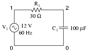
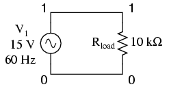
 The .ac card specifies the points of ac analysis from 60Hz to 60Hz, at a single point. This card, of course, is a bit more useful for multi-frequency analysis, where a range of frequencies can be analyzed in steps. The .print card outputs the AC voltage between nodes 1 and 2, and the AC voltage between node 2 and ground. 


 Netlist: 
  
Demo of a simple AC circuit
v1 1 0 ac 12 sin
r1 1 2 30
c1 2 0 100u
.ac lin 1 60 60
.print ac v(1,2) v(2)
.end


 Output: 
  
freq          v(1,2)      v(2)   
6.000E+01     8.990E+00   7.949E+00
         
Low-pass filter
  
  
   
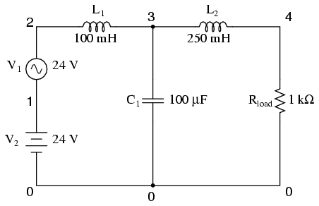
 This low-pass filter blocks AC and passes DC to the Rload resistor. Typical of a filter used to suppress ripple from a rectifier circuit, it actually has a resonant frequency, technically making it a band-pass filter. However, it works well anyway to pass DC and block the high-frequency harmonics generated by the AC-to-DC rectification process. Its performance is measured with an AC source sweeping from 500 Hz to 15 kHz. If desired, the .print card can be substituted or supplemented with a .plot card to show AC voltage at node 4 graphically. 


 Netlist: 
  
Lowpass filter
v1 2 1 ac 24 sin
v2 1 0 dc 24
rload 4 0 1k
l1 2 3 100m
l2 3 4 250m
c1 3 0 100u
.ac lin 30 500 15k
.print ac v(4)
.plot ac v(4)
.end


freq          v(4)       
5.000E+02     1.935E-01
1.000E+03     3.275E-02
1.500E+03     1.057E-02
2.000E+03     4.614E-03
2.500E+03     2.402E-03
3.000E+03     1.403E-03
3.500E+03     8.884E-04
4.000E+03     5.973E-04
4.500E+03     4.206E-04
5.000E+03     3.072E-04
5.500E+03     2.311E-04
6.000E+03     1.782E-04
6.500E+03     1.403E-04
7.000E+03     1.124E-04
7.500E+03     9.141E-05
8.000E+03     7.536E-05
8.500E+03     6.285E-05
9.000E+03     5.296E-05
9.500E+03     4.504E-05
1.000E+04     3.863E-05
1.050E+04     3.337E-05
1.100E+04     2.903E-05
1.150E+04     2.541E-05
1.200E+04     2.237E-05
1.250E+04     1.979E-05
1.300E+04     1.760E-05
1.350E+04     1.571E-05
1.400E+04     1.409E-05
1.450E+04     1.268E-05
1.500E+04     1.146E-05


freq       v(4)  1.000E-06     1.000E-04    1.000E-02    1.000E+00
- - - - - - - - - - - - - - - - - - - - - - - - - - - - - - - - - -
5.000E+02  1.935E-01 .             .             .        *    .
1.000E+03  3.275E-02 .             .             .   *         .
1.500E+03  1.057E-02 .             .             *             .
2.000E+03  4.614E-03 .             .           * .             .
2.500E+03  2.402E-03 .             .         *   .             .
3.000E+03  1.403E-03 .             .       *     .             .
3.500E+03  8.884E-04 .             .      *      .             .
4.000E+03  5.973E-04 .             .    *        .             .
4.500E+03  4.206E-04 .             .   *         .             .
5.000E+03  3.072E-04 .             .  *          .             .
5.500E+03  2.311E-04 .             .  *          .             .
6.000E+03  1.782E-04 .             . *           .             .
6.500E+03  1.403E-04 .             .*            .             .
7.000E+03  1.124E-04 .             *             .             .
7.500E+03  9.141E-05 .             *             .             .
8.000E+03  7.536E-05 .            *.             .             .
8.500E+03  6.285E-05 .            *.             .             .
9.000E+03  5.296E-05 .           * .             .             .
9.500E+03  4.504E-05 .           * .             .             .
1.000E+04  3.863E-05 .          *  .             .             .
1.050E+04  3.337E-05 .          *  .             .             .
1.100E+04  2.903E-05 .         *   .             .             .
1.150E+04  2.541E-05 .         *   .             .             .
1.200E+04  2.237E-05 .        *    .             .             .
1.250E+04  1.979E-05 .        *    .             .             .
1.300E+04  1.760E-05 .        *    .             .             .
1.350E+04  1.571E-05 .       *     .             .             .
1.400E+04  1.409E-05 .       *     .             .             .
1.450E+04  1.268E-05 .       *     .             .             .
1.500E+04  1.146E-05 .      *      .             .             .
- - - - - - - - - - - - - - - - - - - - - - - - - - - - - - - - - -
       
Multiple-source AC network
  
  
   
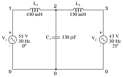
 One of the idiosyncrasies of SPICE is its inability to handle any loop in a circuit exclusively composed of series voltage sources and inductors. Therefore, the "loop" of V1-L1-L2-V2-V1 is unacceptable.  To get around this, I had to insert a low-resistance resistor somewhere in that loop to break it up.  Thus, we have Rbogus between 3 and 4 (with 1 pico-ohm of resistance), and V2 between 4 and 0.  The circuit above is the original design, while the circuit below has Rbogus inserted to avoid the SPICE error.   
  
  


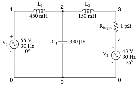
 Netlist: 
  
Multiple ac source
v1 1 0 ac 55 0 sin
v2 4 0 ac 43 25 sin
l1 1 2 450m
c1 2 0 330u
l2 2 3 150m
rbogus 3 4 1e-12
.ac lin 1 30 30
.print ac v(2)
.end


 Output: 
  
freq          v(2)       
3.000E+01     1.413E+02
        
AC phase shift demonstration
  
  
   
 The currents through each leg are indicated by the voltage drops across each respective shunt resistor (1 amp = 1 volt through 1 Ω), output by the v(1,2) and v(1,3) terms of the .print card. The phase of the currents through each leg are indicated by the phase of the voltage drops across each respective shunt resistor, output by the vp(1,2) and vp(1,3) terms in the .print card. 


 Netlist: 
  
phase shift
v1 1 0 ac 4 sin
rshunt1 1 2 1
rshunt2 1 3 1
l1 2 0 1
r1 3 0 6.3k
.ac lin 1 1000 1000
.print ac v(1,2) v(1,3) vp(1,2) vp(1,3)
.end


 Output: 
  
freq          v(1,2)      v(1,3)      vp(1,2)     vp(1,3)
1.000E+03     6.366E-04   6.349E-04  -9.000E+01   0.000E+00
        
Transformer circuit
  
  
   
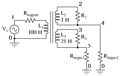
 SPICE understands transformers as a set of mutually coupled inductors. Thus, to simulate a transformer in SPICE, you must specify the primary and secondary windings as separate inductors, then instruct SPICE to link them together with a "k" card specifying the coupling constant. For ideal transformer simulation, the coupling constant would be unity (1). However, SPICE can't handle this value, so we use something like 0.999 as the coupling factor. 
  
 Note that all winding inductor pairs must be coupled with their own k cards in order for the simulation to work properly.  For a two-winding transformer, a single k card will suffice.  For a three-winding transformer, three k cards must be specified (to link L1 with L2, L2 with L3, and L1 with L3). 
  
 The L1/L2 inductance ratio of 100:1 provides a 10:1 step-down voltage transformation ratio. With 120 volts in we should see 12 volts out of the L2 winding.  The L1/L3 inductance ratio of 100:25 (4:1) provides a 2:1 step-down voltage transformation ratio, which should give us 60 volts out of the L3 winding with 120 volts in. 


 Netlist: 
  
transformer                                                                
v1 1 0 ac 120 sin  
rbogus0 1 6 1e-3
l1 6 0 100 
l2 2 4 1
l3 3 5 25  
k1 l1 l2 0.999
k2 l2 l3 0.999
k3 l1 l3 0.999
r1 2 4 1000
r2 3 5 1000
rbogus1 5 0 1e10
rbogus2 4 0 1e10
.ac lin 1 60 60
.print ac v(1,0) v(2,0) v(3,0)
.end


 Output: 
  
freq          v(1)        v(2)        v(3)       
6.000E+01     1.200E+02   1.199E+01   5.993E+01
  
 In this example, Rbogus0 is a very low-value resistor, serving to break up the source/inductor loop of V1/L1.  Rbogus1 and Rbogus2 are very high-value resistors necessary to provide DC paths to ground on each of the isolated circuits. Note as well that one side of the primary circuit is directly grounded. Without these ground references, SPICE will produce errors! 
        
Full-wave bridge rectifier
  
  
   
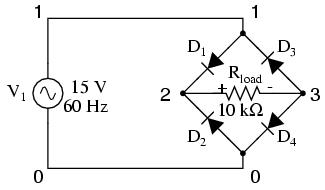
Diodes, like all semiconductor components in SPICE, must be modeled so that SPICE knows all the nitty-gritty details of how they're supposed to work. Fortunately, SPICE comes with a few generic models, and the diode is the most basic. Notice the .model card which simply specifies "d" as the generic diode model for mod1. Again, since we're plotting the waveforms here, we need to specify all parameters of the AC source in a single card and print/plot all values using the .tran option. 


 Netlist: 
  
fullwave bridge rectifier
v1 1 0 sin(0 15 60 0 0)
rload 1 0 10k
d1 1 2 mod1
d2 0 2 mod1
d3 3 1 mod1
d4 3 0 mod1
.model mod1 d
.tran .5m 25m
.plot tran v(1,0) v(2,3)
.end


 Output: 
  
legend:

*: v(1)
+: v(2,3)

time      v(1)

(*)--------- -2.000E+01  -1.000E+01   0.000E+00   1.000E+01  2.000E+01
(+)--------- -5.000E+00   0.000E+00   5.000E+00   1.000E+01  1.500E+01
- - - - - - - - - - - - - - - - - - - - - - - - - - - - - - - - - -
0.000E+00  0.000E+00 .       +            *            .           .
5.000E-04  2.806E+00 .       .      +     .   *        .           .
1.000E-03  5.483E+00 .       .            +      *     .           .
1.500E-03  7.929E+00 .       .            .     +   *  .           .
2.000E-03  1.013E+01 .       .            .           +*           .
2.500E-03  1.198E+01 .       .            .            .  * +      .
3.000E-03  1.338E+01 .       .            .            .    *  +   .
3.500E-03  1.435E+01 .       .            .            .     *    +.
4.000E-03  1.476E+01 .       .            .            .      *    +
4.500E-03  1.470E+01 .       .            .            .      *    +
5.000E-03  1.406E+01 .       .            .            .     *   + .
5.500E-03  1.299E+01 .       .            .            .   *  +    .
6.000E-03  1.139E+01 .       .            .            . *+        .
6.500E-03  9.455E+00 .       .            .         + *.           .
7.000E-03  7.113E+00 .       .            .   +    *   .           .
7.500E-03  4.591E+00 .       .           +.    *       .           .
8.000E-03  1.841E+00 .       .   +        . *          .           .
8.500E-03 -9.177E-01 .       .  +        *.            .           .
9.000E-03 -3.689E+00 .       .        *+  .            .           .
9.500E-03 -6.380E+00 .       .    *       . +          .           .
1.000E-02 -8.784E+00 .       . *          .        +   .           .
1.050E-02 -1.075E+01 .      *.            .            .+          .
1.100E-02 -1.255E+01 .   *   .            .            .     +     .
1.150E-02 -1.372E+01 .  *    .            .            .        +  .
1.200E-02 -1.460E+01 . *     .            .            .           +
1.250E-02 -1.476E+01 .*      .            .            .           +
1.300E-02 -1.460E+01 . *     .            .            .           +
1.350E-02 -1.373E+01 .  *    .            .            .        +  .
1.400E-02 -1.254E+01 .   *   .            .            .     +     .
1.450E-02 -1.077E+01 .      *.            .            .+          .
1.500E-02 -8.726E+00 .       . *          .       +    .           .
1.550E-02 -6.293E+00 .       .    *       . +          .           .
1.600E-02 -3.684E+00 .       .        x   .            .           .
1.650E-02 -9.361E-01 .       .      +    *.            .           .
1.700E-02  1.875E+00 .       .      +     . *          .           .
1.750E-02  4.552E+00 .       .           +.    *       .           .
1.800E-02  7.170E+00 .       .            .   +    *   .           .
1.850E-02  9.401E+00 .       .            .         + *.           .
1.900E-02  1.146E+01 .       .            .            . *+        .
1.950E-02  1.293E+01 .       .            .            .   *  +    .
2.000E-02  1.414E+01 .       .            .            .     *    +.
2.050E-02  1.464E+01 .       .            .            .     *     +
2.100E-02  1.483E+01 .       .            .            .      *    +
2.150E-02  1.430E+01 .       .            .            .     *    +.
2.200E-02  1.344E+01 .       .            .            .    *   +  .
2.250E-02  1.195E+01 .       .            .            .  *+       .
2.300E-02  1.016E+01 .       .            .           +*           .
2.350E-02  7.917E+00 .       .            .     +   *  .           .
2.400E-02  5.460E+00 .       .            +      *     .           .
2.450E-02  2.809E+00 .       .      +     .  *         .           .
2.500E-02 -8.297E-04 .       +            *            .           .
- - - - - - - - - - - - - - - - - - - - - - - - - - - - - - - - - -
         
Common-base BJT transistor amplifier
  
  
   
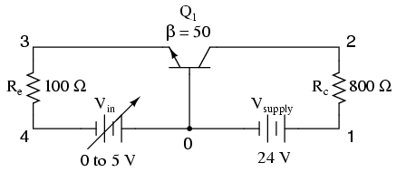
 This analysis sweeps the input voltage (Vin) from 0 to 5 volts in 0.1 volt increments, then prints out the voltage between the collector and emitter leads of the transistor v(2,3). The transistor (Q1) is an NPN with a forward Beta of 50. 


 Netlist: 
  
Common-base BJT amplifier
vsupply 1 0 dc 24
vin 0 4 dc
rc 1 2 800
re 3 4 100
q1 2 0 3 mod1
.model mod1 npn bf=50
.dc vin 0 5 0.1
.print dc v(2,3)
.plot dc v(2,3)
.end


 Output: 
  
vin           v(2,3)     
0.000E+00     2.400E+01
1.000E-01     2.410E+01
2.000E-01     2.420E+01
3.000E-01     2.430E+01
4.000E-01     2.440E+01
5.000E-01     2.450E+01
6.000E-01     2.460E+01
7.000E-01     2.466E+01
8.000E-01     2.439E+01
9.000E-01     2.383E+01
1.000E+00     2.317E+01
1.100E+00     2.246E+01
1.200E+00     2.174E+01
1.300E+00     2.101E+01
1.400E+00     2.026E+01
1.500E+00     1.951E+01
1.600E+00     1.876E+01
1.700E+00     1.800E+01
1.800E+00     1.724E+01
1.900E+00     1.648E+01
2.000E+00     1.572E+01
2.100E+00     1.495E+01
2.200E+00     1.418E+01
2.300E+00     1.342E+01
2.400E+00     1.265E+01
2.500E+00     1.188E+01
2.600E+00     1.110E+01
2.700E+00     1.033E+01
2.800E+00     9.560E+00
2.900E+00     8.787E+00
3.000E+00     8.014E+00
3.100E+00     7.240E+00
3.200E+00     6.465E+00
3.300E+00     5.691E+00
3.400E+00     4.915E+00
3.500E+00     4.140E+00
3.600E+00     3.364E+00
3.700E+00     2.588E+00
3.800E+00     1.811E+00
3.900E+00     1.034E+00
4.000E+00     2.587E-01
4.100E+00     9.744E-02
4.200E+00     7.815E-02
4.300E+00     6.806E-02
4.400E+00     6.141E-02
4.500E+00     5.657E-02
4.600E+00     5.281E-02
4.700E+00     4.981E-02
4.800E+00     4.734E-02
4.900E+00     4.525E-02
5.000E+00     4.346E-02


vin        v(2,3) 0.000E+00    1.000E+01    2.000E+01     3.000E+01
- - - - - - - - - - - - - - - - - - - - - - - - - - - - - - - - - -
0.000E+00  2.400E+01 .             .             .     *       .
1.000E-01  2.410E+01 .             .             .     *       .
2.000E-01  2.420E+01 .             .             .     *       .
3.000E-01  2.430E+01 .             .             .     *       .
4.000E-01  2.440E+01 .             .             .     *       .
5.000E-01  2.450E+01 .             .             .     *       .
6.000E-01  2.460E+01 .             .             .     *       .
7.000E-01  2.466E+01 .             .             .      *      .
8.000E-01  2.439E+01 .             .             .     *       .
9.000E-01  2.383E+01 .             .             .    *        .
1.000E+00  2.317E+01 .             .             .   *         .
1.100E+00  2.246E+01 .             .             .  *          .
1.200E+00  2.174E+01 .             .             . *           .
1.300E+00  2.101E+01 .             .             .*            .
1.400E+00  2.026E+01 .             .             *             .
1.500E+00  1.951E+01 .             .            *.             .
1.600E+00  1.876E+01 .             .           * .             .
1.700E+00  1.800E+01 .             .          *  .             .
1.800E+00  1.724E+01 .             .         *   .             .
1.900E+00  1.648E+01 .             .        *    .             .
2.000E+00  1.572E+01 .             .       *     .             .
2.100E+00  1.495E+01 .             .      *      .             .
2.200E+00  1.418E+01 .             .     *       .             .
2.300E+00  1.342E+01 .             .    *        .             .
2.400E+00  1.265E+01 .             .   *         .             .
2.500E+00  1.188E+01 .             .  *          .             . 
2.600E+00  1.110E+01 .             . *           .             .
2.700E+00  1.033E+01 .             *             .             .
2.800E+00  9.560E+00 .            *.             .             .
2.900E+00  8.787E+00 .           * .             .             .
3.000E+00  8.014E+00 .          *  .             .             .
3.100E+00  7.240E+00 .         *   .             .             .
3.200E+00  6.465E+00 .        *    .             .             .
3.300E+00  5.691E+00 .       *     .             .             .
3.400E+00  4.915E+00 .      *      .             .             .
3.500E+00  4.140E+00 .     *       .             .             .
3.600E+00  3.364E+00 .    *        .             .             .
3.700E+00  2.588E+00 .   *         .             .             .
3.800E+00  1.811E+00 .  *          .             .             .
3.900E+00  1.034E+00 .*            .             .             .
4.000E+00  2.587E-01 *             .             .             .
4.100E+00  9.744E-02 *             .             .             .
4.200E+00  7.815E-02 *             .             .             .
4.300E+00  6.806E-02 *             .             .             .
4.400E+00  6.141E-02 *             .             .             .
4.500E+00  5.657E-02 *             .             .             .
4.600E+00  5.281E-02 *             .             .             .
4.700E+00  4.981E-02 *             .             .             .
4.800E+00  4.734E-02 *             .             .             .
4.900E+00  4.525E-02 *             .             .             .
5.000E+00  4.346E-02 *             .             .             .        
- - - - - - - - - - - - - - - - - - - - - - - - - - - - - - - - - -
        
Common-source JFET amplifier with self-bias
  
  
   
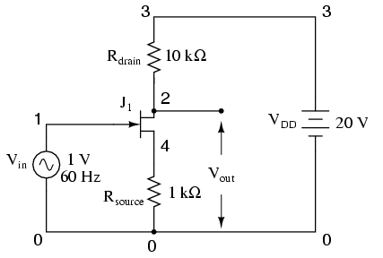
 Netlist: 
  
common source jfet amplifier                  
vin 1 0 sin(0 1 60 0 0)
vdd 3 0 dc 20
rdrain 3 2 10k 
rsource 4 0 1k  
j1 2 1 4 mod1
.model mod1 njf
.tran 1m 30m
.plot tran v(2,0) v(1,0)
.end


 Output: 
  
legend:
*: v(2)
+: v(1)
time      v(2)
(*)---------  1.400E+01    1.600E+01   1.800E+01  2.000E+01 2.200E+01
(+)--------- -1.000E+00   -5.000E-01   0.000E+00  5.000E-01 1.000E+00
- - - - - - - - - - - - - - - - - - - - - - - - - - - - - - - - - -
0.000E+00  1.708E+01 .           .     *    +          .           .
1.000E-03  1.609E+01 .           .*         .        + .           .
2.000E-03  1.516E+01 .       *   .          .          .  +        .
3.000E-03  1.448E+01 .  *        .          .          .        +  .
4.000E-03  1.419E+01 .*          .          .          .           +
5.000E-03  1.432E+01 . *         .          .          .          +.
6.000E-03  1.490E+01 .     *     .          .          .    +      .
7.000E-03  1.577E+01 .         * .          .         +.           .
8.000E-03  1.676E+01 .           .  *       .  +       .           .
9.000E-03  1.768E+01 .           .    +    *.          .           .
1.000E-02  1.841E+01 .         + .          . *        .           .
1.100E-02  1.890E+01 .   +       .          .    *     .           .
1.200E-02  1.912E+01 .+          .          .      *   .           .
1.300E-02  1.912E+01 .+          .          .      *   .           .
1.400E-02  1.890E+01 .   +       .          .    *     .           .
1.500E-02  1.842E+01 .         + .          . *        .           .
1.600E-02  1.768E+01 .           .    +    *.          .           .
1.700E-02  1.676E+01 .           .  *       .  +       .           .
1.800E-02  1.577E+01 .         * .          .         +.           .
1.900E-02  1.491E+01 .     *     .          .          .    +      .
2.000E-02  1.432E+01 . *         .          .          .          +.
2.100E-02  1.419E+01 .*          .          .          .           +
2.200E-02  1.449E+01 .  *        .          .          .        +  .
2.300E-02  1.516E+01 .       *   .          .          .  +        .
2.400E-02  1.609E+01 .           .*         .        + .           .
2.500E-02  1.708E+01 .           .     *    +          .           .
2.600E-02  1.796E+01 .           . +        *          .           .
2.700E-02  1.861E+01 .        +  .          .  *       .           .
2.800E-02  1.900E+01 .  +        .          .     *    .           .
2.900E-02  1.916E+01 +           .          .      *   .           .
3.000E-02  1.908E+01 .+          .          .      *   .           .
- - - - - - - - - - - - - - - - - - - - - - - - - - - - - - - - - -
         
Inverting op-amp circuit
  
  
   
To simulate an ideal operational amplifier in SPICE, we use a voltage-dependent voltage source as a differential amplifier with extremely high gain. The "e" card sets up the dependent voltage source with four nodes, 3 and 0 for voltage output, and 1 and 0 for voltage input. No power supply is needed for the dependent voltage source, unlike a real operational amplifier. The voltage gain is set at 999,000 in this case. The input voltage source (V1) sweeps from 0 to 3.5 volts in 0.05 volt steps. 


 Netlist: 
  
Inverting opamp
v1 2 0 dc
e 3 0 0 1 999k
r1 3 1 3.29k
r2 1 2 1.18k
.dc v1 0 3.5 0.05
.print dc v(3,0)
.end


 Output: 
  
v1            v(3)       
0.000E+00     0.000E+00
5.000E-02    -1.394E-01
1.000E-01    -2.788E-01
1.500E-01    -4.182E-01
2.000E-01    -5.576E-01
2.500E-01    -6.970E-01
3.000E-01    -8.364E-01
3.500E-01    -9.758E-01
4.000E-01    -1.115E+00
4.500E-01    -1.255E+00
5.000E-01    -1.394E+00
5.500E-01    -1.533E+00
6.000E-01    -1.673E+00
6.500E-01    -1.812E+00
7.000E-01    -1.952E+00
7.500E-01    -2.091E+00
8.000E-01    -2.231E+00
8.500E-01    -2.370E+00
9.000E-01    -2.509E+00
9.500E-01    -2.649E+00
1.000E+00    -2.788E+00
1.050E+00    -2.928E+00
1.100E+00    -3.067E+00
1.150E+00    -3.206E+00
1.200E+00    -3.346E+00
1.250E+00    -3.485E+00
1.300E+00    -3.625E+00
1.350E+00    -3.764E+00
1.400E+00    -3.903E+00
1.450E+00    -4.043E+00
1.500E+00    -4.182E+00
1.550E+00    -4.322E+00
1.600E+00    -4.461E+00
1.650E+00    -4.600E+00
1.700E+00    -4.740E+00
1.750E+00    -4.879E+00
1.800E+00    -5.019E+00
1.850E+00    -5.158E+00
1.900E+00    -5.297E+00
1.950E+00    -5.437E+00
2.000E+00    -5.576E+00
2.050E+00    -5.716E+00
2.100E+00    -5.855E+00
2.150E+00    -5.994E+00
2.200E+00    -6.134E+00
2.250E+00    -6.273E+00
2.300E+00    -6.413E+00
2.350E+00    -6.552E+00
2.400E+00    -6.692E+00
2.450E+00    -6.831E+00
2.500E+00    -6.970E+00
2.550E+00    -7.110E+00
2.600E+00    -7.249E+00
2.650E+00    -7.389E+00
2.700E+00    -7.528E+00
2.750E+00    -7.667E+00
2.800E+00    -7.807E+00
2.850E+00    -7.946E+00
2.900E+00    -8.086E+00
2.950E+00    -8.225E+00
3.000E+00    -8.364E+00
3.050E+00    -8.504E+00
3.100E+00    -8.643E+00
3.150E+00    -8.783E+00
3.200E+00    -8.922E+00
3.250E+00    -9.061E+00
3.300E+00    -9.201E+00
3.350E+00    -9.340E+00
3.400E+00    -9.480E+00
3.450E+00    -9.619E+00
3.500E+00    -9.758E+00
          
Noninverting op-amp circuit
  
  
   
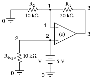
 Another example of a SPICE quirk: since the dependent voltage source "e" isn't considered a load to voltage source V1, SPICE interprets V1 to be open-circuited and will refuse to analyze it.  The fix is to connect Rbogus in parallel with V1 to act as a DC load.  Being directly connected across V1, the resistance of Rbogus is not crucial to the operation of the circuit, so 10 kΩ will work fine.  I decided not to sweep the V1 input voltage at all in this circuit for the sake of keeping the netlist and output listing simple. 


 Netlist: 
  
noninverting opamp
v1 2 0 dc 5
rbogus 2 0 10k
e 3 0 2 1 999k
r1 3 1 20k
r2 1 0 10k
.end


 Output: 
  
node     voltage   node     voltage   node    voltage
(  1)    5.0000    (  2)    5.0000    (  3)   15.0000
         
Instrumentation amplifier
  
  
   
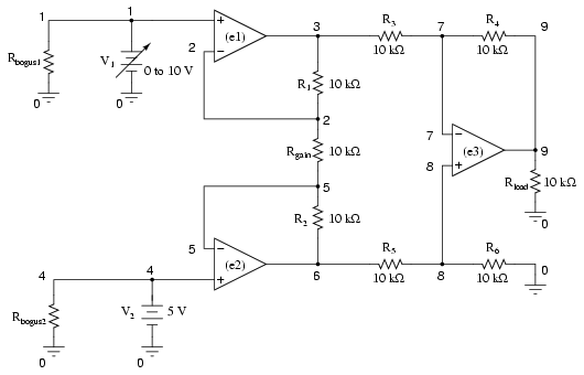
 Note the very high-resistance Rbogus1 and Rbogus2 resistors in the netlist (not shown in schematic for brevity) across each input voltage source, to keep SPICE from thinking V1 and V2 were open-circuited, just like the other op-amp circuit examples. 


 Netlist: 
  
Instrumentation amplifier
v1 1 0
rbogus1 1 0 9e12
v2 4 0 dc 5
rbogus2 4 0 9e12
e1 3 0 1 2 999k
e2 6 0 4 5 999k
e3 9 0 8 7 999k
rload 9 0 10k
r1 2 3 10k
rgain 2 5 10k
r2 5 6 10k
r3 3 7 10k
r4 7 9 10k
r5 6 8 10k
r6 8 0 10k
.dc v1 0 10 1
.print dc v(9) v(3,6)
.end


 Output: 
  
v1            v(9)        v(3,6) 
0.000E+00     1.500E+01  -1.500E+01
1.000E+00     1.200E+01  -1.200E+01
2.000E+00     9.000E+00  -9.000E+00
3.000E+00     6.000E+00  -6.000E+00
4.000E+00     3.000E+00  -3.000E+00
5.000E+00     9.955E-11  -9.956E-11
6.000E+00    -3.000E+00   3.000E+00
7.000E+00    -6.000E+00   6.000E+00
8.000E+00    -9.000E+00   9.000E+00
9.000E+00    -1.200E+01   1.200E+01
1.000E+01    -1.500E+01   1.500E+01
         
Op-amp integrator with sinewave input
  
  


 Netlist: 
  
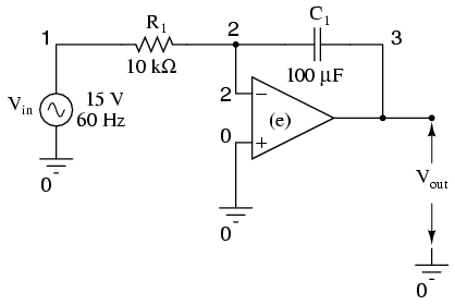
Integrator with sinewave input
vin 1 0 sin (0 15 60 0 0)
r1 1 2 10k
c1 2 3 150u ic=0
e 3 0 0 2 999k
.tran 1m 30m uic
.plot tran v(1,0) v(3,0)
.end


 Output: 
  
legend:
*: v(1)
+: v(3)
time       v(1)
(*)-------- -2.000E+01    -1.000E+01     0.000E+00     1.000E+01
(+)-------- -6.000E-02    -4.000E-02    -2.000E-02     0.000E+00
- - - - - - - - - - - - - - - - - - - - - - - - - - - - - - - - - -
0.000E+00  6.536E-08 .        .             *             +       .
1.000E-03  5.516E+00 .        .             .       *    +.       .
2.000E-03  1.021E+01 .        .             .        +    *       .
3.000E-03  1.350E+01 .        .             .  +          .    *  .
4.000E-03  1.495E+01 .        .          +  .             .      *.
5.000E-03  1.418E+01 .        .   +         .             .     * .
6.000E-03  1.150E+01 .      + .             .             . *     .
7.000E-03  7.214E+00 . +      .             .         *   .       .
8.000E-03  1.867E+00 .+       .             .  *          .       .
9.000E-03 -3.709E+00 . +      .        *    .             .       .
1.000E-02 -8.805E+00 .   +    . *           .             .       .
1.100E-02 -1.259E+01 .    *   +             .             .       .
1.200E-02 -1.466E+01 . *      .     +       .             .       .
1.300E-02 -1.471E+01 . *      .            +.             .       .
1.400E-02 -1.259E+01 .    *   .             .    +        .       .
1.500E-02 -8.774E+00 .        . *           .         +   .       .
1.600E-02 -3.723E+00 .        .        *    .            +.       .
1.700E-02  1.870E+00 .        .             .  *          +       .
1.800E-02  7.188E+00 .        .             .         * + .       .
1.900E-02  1.154E+01 .        .             .      +      . *     .
2.000E-02  1.418E+01 .        .             .+            .     * .
2.100E-02  1.490E+01 .        .       +     .             .      *.
2.200E-02  1.355E+01 .        . +           .             .    *  .
2.300E-02  1.020E+01 .    +   .             .             *       .
2.400E-02  5.496E+00 . +      .             .       *     .       .
2.500E-02 -1.486E-03 .+       .             *             .       .
2.600E-02 -5.489E+00 . +      .     *       .             .       .
2.700E-02 -1.021E+01 .    +   *             .             .       .
2.800E-02 -1.355E+01 .   *    . +           .             .       .
2.900E-02 -1.488E+01 . *      .       +     .             .       .
3.000E-02 -1.427E+01 .  *     .             .+            .       .
- - - - - - - - - - - - - - - - - - - - - - - - - - - - - - - - - -
         
Op-amp integrator with squarewave input
  
  


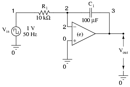
 Netlist: 
  
Integrator with squarewave input
vin 1 0 pulse (-1 1 0 0 0 10m 20m)
r1 1 2 1k
c1 2 3 150u ic=0
e 3 0 0 2 999k
.tran 1m 50m uic
.plot tran v(1,0) v(3,0)
.end


 Output: 
  
legend:
*: v(1)
+: v(3)
time       v(1)
(*)-------- -1.000E+00   -5.000E-01     0.000E+00  5.000E-01  1.000E+00
(+)-------- -1.000E-01   -5.000E-02     0.000E+00  5.000E-02  1.000E-01
- - - - - - - - - - - - - - - - - - - - - - - - - - - - - - - - - -
0.000E+00 -1.000E+00 *         .             +           .         .
1.000E-03  1.000E+00 .         .             +           .         *
2.000E-03  1.000E+00 .         .           + .           .         *
3.000E-03  1.000E+00 .         .         +   .           .         *
4.000E-03  1.000E+00 .         .       +     .           .         *
5.000E-03  1.000E+00 .         .      +      .           .         *
6.000E-03  1.000E+00 .         .    +        .           .         *
7.000E-03  1.000E+00 .         .  +          .           .         *
8.000E-03  1.000E+00 .         .+            .           .         *
9.000E-03  1.000E+00 .        +.             .           .         *
1.000E-02  1.000E+00 .      +  .             .           .         *
1.100E-02  1.000E+00 .    +    .             .           .         *
1.200E-02 -1.000E+00 *    +    .             .           .         .
1.300E-02 -1.000E+00 *      +  .             .           .         .
1.400E-02 -1.000E+00 *        +.             .           .         .
1.500E-02 -1.000E+00 *         .+            .           .         .
1.600E-02 -1.000E+00 *         .  +          .           .         .
1.700E-02 -1.000E+00 *         .    +        .           .         .
1.800E-02 -1.000E+00 *         .      +      .           .         .
1.900E-02 -1.000E+00 *         .       +     .           .         .
2.000E-02 -1.000E+00 *         .         +   .           .         .
2.100E-02  1.000E+00 .         .         +   .           .         *
2.200E-02  1.000E+00 .         .       +     .           .         *
2.300E-02  1.000E+00 .         .      +      .           .         *
2.400E-02  1.000E+00 .         .    +        .           .         *
2.500E-02  1.000E+00 .         .  +          .           .         *
2.600E-02  1.000E+00 .         .+            .           .         *
2.700E-02  1.000E+00 .        +.             .           .         *
2.800E-02  1.000E+00 .      +  .             .           .         *
2.900E-02  1.000E+00 .    +    .             .           .         *
3.000E-02  1.000E+00 .  +      .             .           .         *
3.100E-02  1.000E+00 . +       .             .           .         *
3.200E-02 -1.000E+00 * +       .             .           .         .
3.300E-02 -1.000E+00 *  +      .             .           .         .
3.400E-02 -1.000E+00 *    +    .             .           .         .
3.500E-02 -1.000E+00 *      +  .             .           .         .
3.600E-02 -1.000E+00 *        +.             .           .         .
3.700E-02 -1.000E+00 *         .+            .           .         .
3.800E-02 -1.000E+00 *         .  +          .           .         .
3.900E-02 -1.000E+00 *         .    +        .           .         .
4.000E-02 -1.000E+00 *         .      +      .           .         .
4.100E-02  1.000E+00 .         .      +      .           .         *
4.200E-02  1.000E+00 .         .    +        .           .         *
4.300E-02  1.000E+00 .         .  +          .           .         *
4.400E-02  1.000E+00 .         .+            .           .         *
4.500E-02  1.000E+00 .        +.             .           .         *
4.600E-02  1.000E+00 .      +  .             .           .         *
4.700E-02  1.000E+00 .    +    .             .           .         *
4.800E-02  1.000E+00 .  +      .             .           .         *
4.900E-02  1.000E+00 . +       .             .           .         *
5.000E-02  1.000E+00 +         .             .           .         *
- - - - - - - - - - - - - - - - - - - - - - - - - - - - - - - - - -

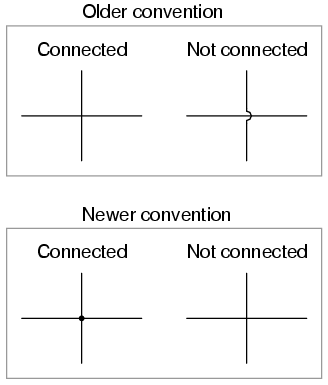
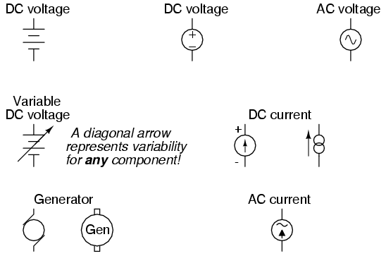
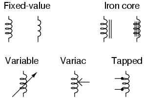
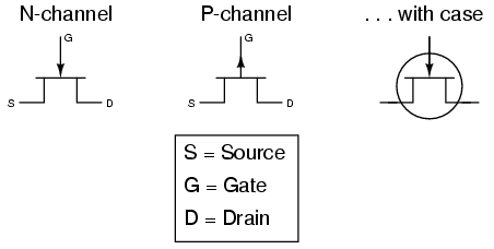
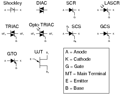
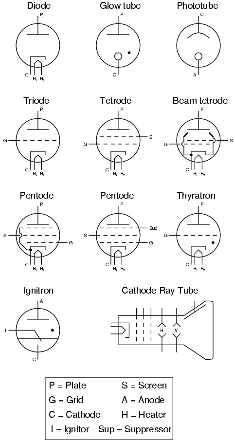
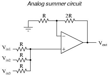READ MORE...